Argument values z under which f(z) goes to zero called. zero point, i.e. if f(a) = 0 , then a - zero point.
Def. Dot a called order zeron
, if
FKP can be represented in the form f(z) = , where  analytic function and
 0.
0.
In this case, in the expansion of the function in a Taylor series (43), the first n coefficients are zero
=
=
Etc. Determine the order of zero for  and (1-cos z) at z
=
0
and (1-cos z) at z
=
0
 =
=
 =
=

 zero 1st order
1 - cos z
=
 =
=
 zero 2nd order
Def. Dot z
=
 called point at infinity and zero functions f(z), if f(
 ) = 0. Such a function expands into a series in negative powers z
: f(z)
=
) = 0. Such a function expands into a series in negative powers z
: f(z)
=
 . If
first n
coefficients are equal to zero, then we arrive at zero order n
at a point at infinity: f(z)
= z
-
n
. If
first n
coefficients are equal to zero, then we arrive at zero order n
at a point at infinity: f(z)
= z
-
n
 .
.
Isolated singular points are divided into: a) removable singular points; b) order polesn; v) essential singular points.
Dot a called removable singular point functions f(z) if z  a
lim f(z)
= With - finite number .
a
lim f(z)
= With - finite number .
Dot a called pole of ordern
(n
 1) features f(z) if the inverse function
  =
1/
f(z) has order zero n at the point a. Such a function can always be represented as f(z)
=
=
1/
f(z) has order zero n at the point a. Such a function can always be represented as f(z)
=
 , where
  - analytical function and
  .
.
Dot a called essential point functions f(z), if z  a
lim f(z) does not exist.
a
lim f(z) does not exist.
Laurent series

Consider the case of an annular convergence region r < | z 0 – a| < R centered on a point a for function f(z). We introduce two new circles L 1 (r) and L 2 (R) near the boundaries of the ring with a dot z 0 between them. Let us make a section of the ring, join the circles along the edges of the section, pass to a simply connected region, and in
Cauchy integral formula (39) we obtain two integrals over the variable z
f(z 0)
=
 +
+
 ,
(42)
,
(42)
where integration goes in opposite directions.
For the integral over L 1 the condition | z 0 – a | > | z – a |, and for the integral over L 2 reverse condition | z 0 – a | < | z – a |. Therefore, the factor 1/( z – z 0) expand in a series (a) in the integral over L 2 and in series (b) in the integral over L one . As a result, we get the decomposition f(z) in the annular region in Laurent series in positive and negative powers ( z 0 – a)
f(z 0)
=
 A n
(z 0 – a) n
(43)
A n
(z 0 – a) n
(43)
where A n
=
 =
= ;A -n
=
;A -n
=
Expansion in positive powers (z 0 - a) called right part Laurent series (Taylor series), and the expansion in negative powers is called. main part Laurent row.
If inside the circle L 1 there are no singular points and the function is analytic, then in (44) the first integral is equal to zero by the Cauchy theorem, and only the correct part remains in the expansion of the function. Negative powers in expansion (45) appear only when analyticity is violated within the inner circle and serve to describe the function near isolated singular points.
To construct the Laurent series (45) for f(z) one can calculate the expansion coefficients according to the general formula or use the expansions of the elementary functions included in f(z).
Number of terms ( n) of the main part of the Laurent series depends on the type of singular point: removable singular point
(n
=
0)
; essential singular point
(n  );
polen-th order(n
-
end number).
);
polen-th order(n
-
end number).
and for f(z)
=
 dot z
= 0 removable singular point, because there is no main part. f(z)
=
(z
-
dot z
= 0 removable singular point, because there is no main part. f(z)
=
(z
-
 ) = 1 -

b) For f(z)
=
 dot z
= 0 -
1st order pole
dot z
= 0 -
1st order pole
f(z)
=
 (z
-
(z
-
 ) =
-
) =
-

c) For f(z) = e 1 / z dot z = 0 - essential singular point
f(z)
=
e 1 /
z =

If f(z) is analytic in the domain D with the exception of m isolated singular points  and | z 1 |
< |z 2 |
< . . . < |z m| , then when expanding the function in powers z the whole plane is divided into m+ 1 ring | z i |
< | z
| < | z i+ 1 | and the Laurent series has a different form for each ring. When expanding in powers ( z
–
z i
) the convergence region of the Laurent series is the circle | z
–
z i
| < r, where r
is the distance to the nearest singular point.
and | z 1 |
< |z 2 |
< . . . < |z m| , then when expanding the function in powers z the whole plane is divided into m+ 1 ring | z i |
< | z
| < | z i+ 1 | and the Laurent series has a different form for each ring. When expanding in powers ( z
–
z i
) the convergence region of the Laurent series is the circle | z
–
z i
| < r, where r
is the distance to the nearest singular point.
Etc. Expand the function f(z)
= in Laurent's series in powers z and ( z
-
1).
in Laurent's series in powers z and ( z
-
1).
Solution. We represent the function in the form f(z)
= - z 2
 . We use the formula for the sum of a geometric progression
  . In the circle |z|< 1 ряд сходится и f(z)
= - z 2
(1 + z
+ z 2
+ z 3
+ z 4
+ . . .) = - z 2
- z 3
- z 4 - . . . , i.e. decomposition contains only correct part. Let's move to the outer region of the circle |z| > 1 . We represent the function in the form
. In the circle |z|< 1 ряд сходится и f(z)
= - z 2
(1 + z
+ z 2
+ z 3
+ z 4
+ . . .) = - z 2
- z 3
- z 4 - . . . , i.e. decomposition contains only correct part. Let's move to the outer region of the circle |z| > 1 . We represent the function in the form  , where 1/| z|
< 1, и получим разложение f(z)
= z
, where 1/| z|
< 1, и получим разложение f(z)
= z =z
+ 1 +
=z
+ 1 +

Because , expansion of the function in powers ( z
-
1) looks like f(z)
= (z
-
1) -1
+ 2 + (z
-
1) for everyone  1.
1.
Etc. Expand the function in a Laurent series f(z)
=
 :
a) in degrees z in a circle | z|
< 1; b)
по степеням z
ring 1<
|z|
< 3 ; c)
по степеням (z
–
2).Decision. Let's decompose the function into simple fractions
:
a) in degrees z in a circle | z|
< 1; b)
по степеням z
ring 1<
|z|
< 3 ; c)
по степеням (z
–
2).Decision. Let's decompose the function into simple fractions
 =
=
=
= +
+ =
= .
From conditions z
=1
.
From conditions z
=1
 A
= -1/2 , z
=3
A
= -1/2 , z
=3
 B
= ½.
B
= ½.
a) f(z)
=
½ [  ]
= ½ [
]
= ½ [  -(1/3)
 ], when | z|<
1.
], when | z|<
1.
b) f(z)
= - ½ [  +
+ ]
= -
(
]
= -
( ), at 1< |z|
< 3.
), at 1< |z|
< 3.
With) f(z)
=
½ [  ]= -
½
[
]= -
½
[  ]
=
]
=
=
- ½
= -
 , for |2 - z|
< 1
, for |2 - z|
< 1
It is a circle of radius 1 centered on a point z = 2 .
In some cases, power series can be reduced to a set of geometric progressions, and then it is easy to determine the area of their convergence.
Etc. Investigate the convergence of a series
.
. . +
 +
+
 +
+
 +
1
+ ()
+ ()
2
+ ()
3
+ . . .
+
1
+ ()
+ ()
2
+ ()
3
+ . . .
Solution. It is the sum of two geometric progressions with q 1
=
 , q 2 = () . From the conditions of their convergence it follows
  < 1 ,
< 1 ,
 < 1 или |z|
> 1 , |z|
< 2 , т.е. область сходимости ряда кольцо
1 < |z|
< 2 .
< 1 или |z|
> 1 , |z|
< 2 , т.е. область сходимости ряда кольцо
1 < |z|
< 2 .
Function is one of the most important mathematical concepts. Function - variable dependency at from a variable x, if each value X matches a single value at. variable X called the independent variable or argument. variable at called the dependent variable. All values of the independent variable (variable x) form the domain of the function. All values that the dependent variable takes (variable y), form the range of the function.
Function Graph they call the set of all points of the coordinate plane, the abscissas of which are equal to the values of the argument, and the ordinates are equal to the corresponding values of the function, that is, the values of the variable are plotted along the abscissa axis x, and the values of the variable are plotted along the y-axis y. To plot a function, you need to know the properties of the function. The main properties of the function will be discussed below!
To plot a function graph, we recommend using our program - Graphing Functions Online. If you have any questions while studying the material on this page, you can always ask them on our forum. Also on the forum you will be helped to solve problems in mathematics, chemistry, geometry, probability theory and many other subjects!
Basic properties of functions.
1) Function scope and function range.
The scope of a function is the set of all valid values of the argument x(variable x) for which the function y = f(x) defined.
The range of a function is the set of all real values y that the function accepts.
In elementary mathematics, functions are studied only on the set of real numbers.
2) Function zeros.
Zero of the function is the value of the argument at which the value of the function is equal to zero.
3) Intervals of sign constancy of a function.
The intervals of constant sign of a function are such sets of argument values on which the values of the function are only positive or only negative.
4) Monotonicity of the function.
Increasing function (in some interval) - a function in which a larger value of the argument from this interval corresponds to a larger value of the function.
Decreasing function (in some interval) - a function in which a larger value of the argument from this interval corresponds to a smaller value of the function.
5) Even (odd) functions.
An even function is a function whose domain of definition is symmetric with respect to the origin and for any X from the domain of definition the equality f(-x) = f(x). The graph of an even function is symmetrical about the y-axis.
An odd function is a function whose domain of definition is symmetric with respect to the origin and for any X from the domain of definition the equality f(-x) = - f(x). The graph of an odd function is symmetrical about the origin.
6) Limited and unlimited functions.
A function is called bounded if there exists a positive number M such that |f(x)| ≤ M for all values of x . If there is no such number, then the function is unbounded.
7) Periodicity of the function.
A function f(x) is periodic if there exists a non-zero number T such that for any x f(x+T) = f(x). This smallest number is called the period of the function. All trigonometric functions are periodic. (Trigonometric formulas).
Having studied these properties of the function, you can easily explore the function and, using the properties of the function, you can plot the graph of the function. Also look at the material about the truth table, the multiplication table, the periodic table, the table of derivatives and the table of integrals.
Function zeros
What are function zeros? How to determine the zeros of a function analytically and graphically?
Function zeros are the values of the argument at which the function is equal to zero.
To find the zeros of the function given by the formula y=f(x), we need to solve the equation f(x)=0.
If the equation has no roots, then the function has no zeros.
1) Find the zeros of the linear function y=3x+15.
To find the zeros of the function, we solve the equation 3x+15 =0.
So the zero of the function is y=3x+15 - x= -5 .
2) Find the zeros of the quadratic function f(x)=x²-7x+12.
To find the zeros of the function, we solve the quadratic equation
Its roots x1=3 and x2=4 are the zeros of this function.
3) Find the zeros of the function
A fraction makes sense if the denominator is different from zero. Therefore, x²-1≠0, x² ≠ 1,x ≠±1. That is, the domain of definition of this function (ODZ)

From the roots of the equation x²+5x+4=0 x1=-1 x2=-4, only x=-4 is included in the domain of definition.
To find the zeros of a function given graphically, it is necessary to find the points of intersection of the graph of the function with the x-axis.
If the graph does not cross the Ox axis, the function has no zeros.

the function whose graph is shown in the figure has four zeros -
In algebra, the problem of finding the zeros of a function occurs both as an independent task and when solving other problems, for example, when studying a function, solving inequalities, etc.
www.algebraclass.ru
Zero function rule

![]()
![]()
Basic concepts and properties of functions
rule (law of) conformity. Monotonic function .
Limited and unlimited functions. Continuous and
discontinuous function . Even and odd functions.
Periodic function. Function period.
Function zeros . Asymptote .
The scope and range of the function. In elementary mathematics, functions are studied only on the set of real numbers R . This means that the function argument can only take on those real values for which the function is defined, i.e. e . it also only accepts real values. A bunch of X all valid valid values of the argument x, for which the function y = f (x) is defined, called function scope. A bunch of Y all real values y that the function accepts is called function range. Now you can give more precise definition features: rule (law of) correspondence between sets X and Y , by which for each element from the set X you can find one and only one element from the set Y, is called a function .
It follows from this definition that a function is considered given if:
- the scope of the function is set X ;
— range of function values is set Y ;
- the rule (law) of correspondence is known, and such that for each
argument values, only one function value can be found.
This requirement of uniqueness of the function is mandatory.
monotonic function.
If for any two values of the argument x 1 and x 2 of the condition x 2 > x 1 follows f (x 2) > f (x 1), then the function f (x) is called increasing; if for any x 1 and x 2 of the condition x 2 > x 1 follows f (x 2) 
The function depicted in Fig. 3 is bounded, but not monotonic. The function in Figure 4 is just the opposite, monotonic but unbounded. (Explain this please!)
Continuous and discontinuous functions. Function y = f (x) is called continuous at the point x = a, if:
1) the function is defined for x = a, i.e. e. f (a) exists;
2) exists finite limit lim f (x) ;
If at least one of these conditions is not met, then the function is called discontinuous at the point x = a .
If the function is continuous in all points of its domain of definition, then it is called continuous function.

Even and odd functions. If for any x from the scope of the function definition takes place: f (— x) = f (x), then the function is called even; if it does: f (— x) = — f (x), then the function is called odd. Graph of an even function symmetrical about the Y axis(Fig.5), a graph of an odd function Sim metric about the origin(Fig. 6).

Periodic function. Function f (x) — periodical if there is such non-zero number T what for any x from the scope of the function definition takes place: f (x + T) = f (x). Such least the number is called function period. All trigonometric functions are periodic.
EXAMPLE 1. Prove that sin x has a period of 2.
SOLUTION We know that sin ( x + 2 n) = sin x, where n= 0, ± 1, ± 2, …
Therefore, adding 2 n to the sine argument
changes its value e . Is there another number with this
Let's pretend that P- such a number, i.e. e. equality:
valid for any value x. But then it has
place and at x= / 2, i.e. e.
sin(/2 + P) = sin / 2 = 1.
But according to the reduction formula sin (/ 2 + P) = cos P. Then
it follows from the last two equalities that cos P= 1, but we
We know that this is only true for P = 2 n. Since the smallest
a non-zero number out of 2 n is 2 , then this number
and there is a period sin x. It is proved similarly that 2
is a period for cos x .
Prove that the functions tan x and cat x have a period.
Example 2. What number is the period of the sin 2 function x ?
Solution. Consider sin 2 x= sin(2 x + 2 n) = sin [ 2 ( x + n) ] .
We see that adding n to the argument x, does not change
function value. Smallest non-zero number
from n is , so this is the period sin 2 x .
Function nulls. The value of the argument for which the function is equal to 0 is called zero ( root) functions. A function can have multiple zeros. For example, the function y = x (x + 1) (x- 3) has three zeros: x = 0, x = — 1, x= 3. Geometrically function null – is the abscissa of the point of intersection of the graph of the function with the axis X .
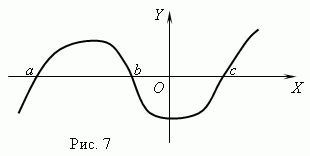
Figure 7 shows the graph of the function with zeros: x = a , x = b and x = c .
Asymptote. If the graph of a function approaches a certain straight line indefinitely as it moves away from the origin, then this straight line is called asymptote.
Topic 6. "Method of intervals".
If f (x) f (x 0) for x x 0, then the function f (x) is called continuous at x 0.
If a function is continuous at every point of some interval I, then it is called continuous on the interval I (the interval I is called function continuity interval). The graph of the function on this interval is a continuous line, which is said to be "drawn without lifting the pencil from the paper."
Property of continuous functions.
If on the interval (a ; b) the function f is continuous and does not vanish, then it retains a constant sign on this interval.
The method of solving inequalities with one variable is based on this property - the method of intervals. Let the function f(x) be continuous on the interval I and vanish at a finite number of points in this interval. By the property of continuous functions, these points divide I into intervals, in each of which the continuous function f(x) c guards a constant sign. To determine this sign, it is enough to calculate the value of the function f(x) at any one point from each such interval. Based on this, we obtain the following algorithm for solving inequalities by the interval method.
The interval method for inequalities of the form
interval method. Average level.
Do you want to test your strength and find out the result of how ready you are for the Unified State Examination or the OGE?
Linear function
A function of the form is called linear. Let's take a function as an example. It is positive at 3″> and negative at. The point is the zero of the function (). Let's show the signs of this function on the real axis:
We say that "the function changes sign when passing through a point".
It can be seen that the signs of the function correspond to the position of the graph of the function: if the graph is above the axis, the sign is “ ”, if it is below it, “ ”.
If we generalize the resulting rule to an arbitrary linear function, we get the following algorithm:
quadratic function
I hope you remember how quadratic inequalities are solved? If not, read the topic "Square inequalities". Let me remind you the general form of a quadratic function: .
Now let's remember what signs the quadratic function takes. Its graph is a parabola, and the function takes the sign “ ” for those in which the parabola is above the axis, and “ ” - if the parabola is below the axis:
If the function has zeros (values at which), the parabola intersects the axis at two points - the roots of the corresponding quadratic equation. Thus, the axis is divided into three intervals, and the signs of the function change alternately when passing through each root.
Is it possible to somehow determine the signs without drawing a parabola each time?
Recall that the square trinomial can be factorized:
Note the roots on the axis:
We remember that the sign of a function can only change when passing through the root. We use this fact: for each of the three intervals into which the axis is divided by roots, it is enough to determine the sign of the function only at one arbitrarily chosen point: at the other points of the interval, the sign will be the same.
In our example: for 3″> both expressions in brackets are positive (we substitute, for example: 0″>). We put the sign "" on the axis:
Well, if (substitute, for example) both brackets are negative, then the product is positive:
That's what it is interval method: knowing the signs of the factors on each interval, we determine the sign of the entire product.
Let us also consider cases when the function has no zeros, or it is only one.
If there are none, then there are no roots. This means that there will be no “passage through the root”. This means that the function on the entire number axis takes only one sign. It is easy to determine by substituting it into a function.
If there is only one root, the parabola touches the axis, so the sign of the function does not change when passing through the root. What is the rule for such situations?
If we factor out such a function, we get two identical factors:
And any squared expression is non-negative! Therefore, the sign of the function does not change. In such cases, we will select the root, when passing through which the sign does not change, circling it with a square:
Such a root will be called multiple.
The method of intervals in inequalities
Now any quadratic inequality can be solved without drawing a parabola. It is enough just to place the signs of the quadratic function on the axis, and choose the intervals depending on the inequality sign. For instance:
We measure the roots on the axis and arrange the signs:
We need the part of the axis with the sign ""; since the inequality is not strict, the roots themselves are also included in the solution:
Now consider rational inequality- an inequality, both parts of which are rational expressions (see "Rational Equations").
Example:
All factors except one - - here are "linear", that is, they contain a variable only in the first degree. We need such linear factors to apply the interval method - the sign changes when passing through their roots. But the multiplier has no roots at all. This means that it is always positive (check it yourself), and therefore does not affect the sign of the entire inequality. This means that you can divide the left and right sides of the inequality into it, and thus get rid of it:
Now everything is the same as it was with quadratic inequalities: we determine at what points each of the factors vanishes, mark these points on the axis and arrange the signs. I draw your attention to a very important fact:
In the case of an even number, we proceed in the same way as before: we circle the point with a square and do not change the sign when passing through the root. But in the case of an odd number, this rule is not fulfilled: the sign will still change when passing through the root. Therefore, we do nothing additionally with such a root, as if it is not a multiple of us. The above rules apply to all even and odd powers.
What do we write in the answer?
If the alternation of signs is violated, you need to be very careful, because with non-strict inequality, the answer should include all filled points. But some of them often stand alone, that is, they do not enter the shaded area. In this case, we add them to the response as isolated dots (in curly braces):
Examples (decide for yourself):
Answers:
- If among the factors it is simple - this is the root, because it can be represented as.
.
What are function zeros? The answer is quite simple - this is a mathematical term, which means the domain of a given function, on which its value is zero. Function zeros are also called Function zeros The easiest way to explain what function zeros are is with a few simple examples.
Examples
Consider a simple equation y=x+3. Since the zero of the function is the value of the argument at which y became zero, we substitute 0 on the left side of the equation:
In this case, -3 is the desired zero. For a given function, there is only one root of the equation, but this is not always the case.
Consider another example:
Substitute 0 on the left side of the equation, as in the previous example:
Obviously, in this case, there will be two zeros of the function: x=3 and x=-3. If the equation had an argument of the third degree, there would be three zeros. We can make a simple conclusion that the number of roots of the polynomial corresponds to the maximum degree of the argument in the equation. However, many functions, for example y=x 3 , at first sight contradict this statement. Logic and common sense suggest that this function has only one zero - at the point x=0. But in fact there are three roots, they just all coincide. If you solve the equation in complex form, this becomes obvious. x=0 in this case, the root, the multiplicity of which is 3. In the previous example, the zeros did not match, therefore they had a multiplicity of 1.
Definition algorithm
From the presented examples it is clear how to determine the zeros of the function. The algorithm is always the same:
- Write a function.
- Substitute y or f(x)=0.
- Solve the resulting equation.
The complexity of the last item depends on the degree of the argument of the equation. When solving equations of high degrees, it is especially important to remember that the number of roots of the equation is equal to the maximum power of the argument. This is especially true for trigonometric equations, where dividing both parts by sine or cosine leads to the loss of roots.
Arbitrary degree equations are most easily solved by Horner's method, which was developed specifically for finding the zeros of an arbitrary polynomial.
The value of zeros of functions can be both negative and positive, real or lying in the complex plane, single or multiple. Or there may be no roots of the equation. For example, the function y=8 will not become zero for any x, because it does not depend on this variable.
The equation y=x 2 -16 has two roots, and both lie in the complex plane: x 1 =4i, x 2 =-4i.

Common Mistakes
A common mistake made by schoolchildren who have not yet really figured out what the zeros of a function are is replacing the argument (x) with zero, and not the value (y) of the function. They confidently substitute x = 0 into the equation and, based on this, find y. But this is the wrong approach.
Another mistake, as already mentioned, is the reduction by sine or cosine in the trigonometric equation, which is why one or more zeros of the function are lost. This does not mean that nothing can be reduced in such equations, but these "lost" factors must be taken into account in further calculations.

Graphical representation
You can understand what the zeros of a function are with the help of mathematical programs such as Maple. In it, you can build a graph by specifying the desired number of points and the desired scale. Those points at which the graph crosses the OX axis are the desired zeros. This is one of the most quick ways finding the roots of a polynomial, especially if its order is higher than the third. So if there is a need to regularly perform mathematical calculations, find the roots of polynomials of arbitrary degrees, build graphs, Maple or a similar program will be simply indispensable for performing and verifying calculations.