SQL 2003 syntax is supported on all platforms.
FLOOR (expression)
If you pass a positive number to the function, then the action of the function will be to remove everything after the decimal point.
SELECT FLOOR(100.1) FROM dual;
However, remember that in the case of negative numbers, rounding down corresponds to an increase in the absolute value.
SELECT FLOOR(-100.1) FROM dual;
To get the opposite effect of the FLOOR function, use the CEIL function.
LN
The LN function returns the natural logarithm of a number, that is, the power to which you need to raise the mathematical constant e (approximately 2.718281) to get the given number as a result.
SQL 2003 syntax
LN (expression)
DB2, Oracle, PostgreSQL
The DB2, Oracle, and PostgreSQL platforms support SQL 2003 syntax for the LN function. DB2 and PostgreSQL also support the LOG function as a synonym for LN.
MySQL and SQL Server
MySQL and SQL Server have their own natural log function, LOG.
LOG (expression)
The following Oracle example calculates the natural logarithm of a number that is approximately equal to a mathematical constant.
SELECT LN(2.718281) FROM dual;
To perform the opposite operation, use the EXP function.
MOD
The MOD function returns the remainder after dividing the dividend by the divisor. All platforms support the SQL 2003 MOD statement syntax.
SQL 2003 syntax
MOD (dividend, divisor)
The standard MOD function is designed to get the remainder after dividing the dividend by the divisor. If the divisor is zero, then the dividend is returned.
The following shows how you can use the MOD function in a SELECT statement.
SELECT MOD(12, 5) FROM NUMBERS 2;
POSITION
The POSITION function returns an integer indicating the starting position of the string in the search string.
SQL 2003 syntax
POSITION(line 1 IN line 2)
The standard POSITION function is designed to get the position of the first occurrence of a given string (string!) in the search string (string!). The function returns 0 if the string! does not occur in the string!, and NULL if any of the arguments is NULL.
DB2
DB2 has an equivalent POSSTR function.
MySQL
The MySQL platform supports the POSITION function according to the SQL 2003 standard.
POWER
The POWER function is used to raise a number to a specified power.
SQL 2003 syntax
POWER (base, exponent)
The result of this function is the base raised to the power determined by the indicator. If the base is negative, then the exponent must be an integer.
DB2, Oracle, PostgreSQL and SQL Server
All of these vendors support SQL 2003 syntax.
Oracle
Oracle has an equivalent INSTR function.
PostgreSQL
The PostgreSQL platform supports the POSITION function according to the SQL 2003 standard.
MySQL
The MySQL platform supports this functionality, not this POW keyword.
P0W (base, exponent)
Raising a positive number to a power is fairly obvious.
SELECT POWER(10.3) FROM dual;
Any number raised to the power of 0 is 1.
SELECT POWER(0.0) FROM dual;
A negative exponent shifts the decimal point to the left.
SELECT POWER(10, -3) FROM dual;
SORT
The SQRT function returns the square root of a number.
SQL 2003 syntax
All platforms support SQL 2003 syntax.
SORT (expression)
SELECT SQRT(100) FROM dual;
WIDTH BUCKET
The WIDTH BUCKET function assigns values to the columns of an equal-width histogram.
SQL 2003 syntax
In the following syntax, an expression is a value that is assigned to the column of the histogram. Typically, the expression is based on one or more columns of the table returned by the query.
WIDTH BUCKET(expression, min, max, histogram_columns)
The histogram columns parameter shows the number of histogram columns to be created in the range of values from min to max. The value of the min parameter is included in the range, but the value of the max parameter is not included. The expression value is assigned to one of the histogram columns, after which the function returns the number of the corresponding histogram column. If the expression does not fall within the specified range of columns, the function returns either 0 or max + 1, depending on whether the expression is less than min or greater than or equal to max.
The following example distributes integer values from 1 to 10 between two columns of a histogram.
The next example is more interesting. The 11 values from 1 to 10 are distributed among the three bars of the histogram to illustrate the difference between the min value, which is included in the range, and the max value, which is not included in the range.
SELECT x, WIDTH_BUCKET(x, 1.10.3) FROM pivot;
Pay special attention to the results cX=, X= 9.9 and X-10. The input parameter value by them, i.e. 1 in this example, falls in the first column, indicating the lower end of the range, since column #1 is defined as x >= min. However, the input value of the max parameter is not included in the maximum column. In this example, the number 10 falls into the overflow column, with number max + 1. The value 9.9 falls into column number 3, and this illustrates the rule that the upper bound of the range is defined as x< max.
This article provides a Transact SQL optimization solution for the problem of calculating stock balances. Applied: Partitioning tables and materialized views.
Formulation of the problem
The task must be solved on SQL Server 2014 Enterprise Edition (x64). The company has many warehouses. Each warehouse has several thousand shipments and receipts of products every day. There is a table of movement of goods in the warehouse income / expense. It is necessary to implement:Calculation of the balance for the selected date and time (up to an hour) for all/any warehouses for each product. For analytics, it is necessary to create an object (function, table, view) with the help of which, for the selected date range, display the data of the source table for all warehouses and products and an additional calculation column - the balance in the position warehouse.
These calculations are expected to run on a schedule with different date ranges and should run at a reasonable time. Those. if it is necessary to display a table with balances for the last hour or day, then the execution time should be as fast as possible, as well as if it is necessary to display the same data for the last 3 years, for subsequent loading into an analytical database.
Technical details. The table itself:
Create table dbo.Turnover (id int identity primary key, dt datetime not null, ProductID int not null, StorehouseID int not null, Operation smallint not null check (Operation in (-1,1)), -- +1 stock check , -1 cost from stock Quantity numeric(20,2) not null, Cost money not null)
Dt - Date and time of receipt / write-off to / from the warehouse.
ProductID - Product
StorehouseID - warehouse
Operation - 2 values incoming or outgoing
Quantity - quantity of the product in stock. It can be real if the product is not in pieces, but, for example, in kilograms.
Cost - the cost of a batch of the product.
Problem research
Let's create a completed table. In order for you to test with me and see the results, I propose to create and fill the dbo.Turnover table with a script:If object_id("dbo.Turnover","U") is not null drop table dbo.Turnover; go with times as (select 1 id union all select id+1 from times where id< 10*365*24*60 -- 10 лет * 365 дней * 24 часа * 60 минут = столько минут в 10 лет)
, storehouse as
(select 1 id
union all
select id+1
from storehouse
where id < 100 -- количество складов)
select
identity(int,1,1) id,
dateadd(minute, t.id, convert(datetime,"20060101",120)) dt,
1+abs(convert(int,convert(binary(4),newid()))%1000) ProductID, -- 1000 - количество разных продуктов
s.id StorehouseID,
case when abs(convert(int,convert(binary(4),newid()))%3) in (0,1) then 1 else -1 end Operation, -- какой то приход и расход, из случайных сделаем из 3х вариантов 2 приход 1 расход
1+abs(convert(int,convert(binary(4),newid()))%100) Quantity
into dbo.Turnover
from times t cross join storehouse s
option(maxrecursion 0);
go
--- 15 min
alter table dbo.Turnover alter column id int not null
go
alter table dbo.Turnover add constraint pk_turnover primary key (id) with(data_compression=page)
go
-- 6 min
I ran this script on a PC with an SSD drive for about 22 minutes, and the table size took about 8GB on the hard drive. You can reduce the number of years and the number of warehouses in order to reduce the time it takes to create and fill out a table. But I recommend leaving some good amount for evaluating query plans, at least 1-2 gigabytes.
Grouping data up to an hour
Next, we need to group the amounts by products in the warehouse for the study period of time, in our formulation of the problem this is one hour (up to a minute, up to 15 minutes, a day is possible. But obviously, up to milliseconds, it is unlikely that anyone will need reporting). For comparisons in the session (window) where we execute our queries, we will execute the command - set statistics time on;. Next, we execute the queries themselves and look at the query plans:
Select top(1000) convert(datetime,convert(varchar(13),dt,120)+":00",120) as dt, -- round to hour ProductID, StorehouseID, sum(Operation*Quantity) as Quantity from dbo .Turnover group by convert(datetime,convert(varchar(13),dt,120)+":00",120), ProductID, StorehouseID
Request cost - 12406
(rows processed: 1000)
SQL Server uptime:
CPU time = 2096594ms, elapsed time = 321797ms.
If we make a resulting query with a balance that is considered a running total of our count, then the query and query plan will be as follows:
Select top(1000) convert(datetime,convert(varchar(13),dt,120)+":00",120) as dt, -- round to hour ProductID, StorehouseID, sum(Operation*Quantity) as Quantity, sum (sum(Operation*Quantity)) over (partition by StorehouseID, ProductID order by convert(datetime,convert(varchar(13),dt,120)+":00",120)) as Balance from dbo.Turnover group by convert (datetime,convert(varchar(13),dt,120)+":00",120), ProductID, StorehouseID

Request cost - 19329
(rows processed: 1000)
SQL Server uptime:
CPU time = 2413155ms, elapsed time = 344631ms.
Grouping optimization
Everything is quite simple here. The query itself without a running total can be optimized with a materialized view (index view). To build a materialized view, what is summed up should not have a NULL value, we sum(Operation*Quantity) sum(Operation*Quantity), or make each field NOT NULL or add isnull/coalesce to the expression. I propose to create a materialized view.
Create view dbo.TurnoverHour with schemabinding as select convert(datetime,convert(varchar(13),dt,120)+":00",120) as dt, -- round to hour ProductID, StorehouseID, sum(isnull(Operation* Quantity,0)) as Quantity, count_big(*) qty from dbo.Turnover group by convert(datetime,convert(varchar(13),dt,120)+":00",120), ProductID, StorehouseID go
And build a clustered index on it. In the index, we indicate the order of the fields in the same way as in the grouping (the order is not important for grouping, it is important that all the fields of the grouping be in the index) and the cumulative total (the order is important here - first what is in partition by, then what is in order by):
Create unique clustered index uix_TurnoverHour on dbo.TurnoverHour (StorehouseID, ProductID, dt) with (data_compression=page) - 19 min
Now, after building the clustered index, we can re-run the queries by changing the sum aggregation as in the view:
Select top(1000) convert(datetime,convert(varchar(13),dt,120)+":00",120) as dt, -- round to hour ProductID, StorehouseID, sum(isnull(Operation*Quantity,0) ) as Quantity from dbo.Turnover group by convert(datetime,convert(varchar(13),dt,120)+":00",120), ProductID, StorehouseID select top(1000) convert(datetime,convert(varchar(13 ),dt,120)+":00",120) as dt, -- round to the hour ProductID, StorehouseID, sum(isnull(Operation*Quantity,0)) as Quantity, sum(sum(isnull(Operation*Quantity, 0))) over (partition by StorehouseID, ProductID order by convert(datetime,convert(varchar(13),dt,120)+":00",120)) as Balance from dbo.Turnover group by convert(datetime,convert (varchar(13),dt,120)+":00",120), ProductID, StorehouseID
Query plans became:
 Cost 0.008
 Cost 0.01
SQL Server uptime:
CPU time = 31ms, elapsed time = 116ms.
(rows processed: 1000)
SQL Server uptime:
CPU time = 0ms, elapsed time = 151ms.
In total, we see that with an indexed view, the query scans not a table grouping data, but a clustered index in which everything is already grouped. And accordingly, the execution time was reduced from 321797 milliseconds to 116 ms, i.e. 2774 times.
This could be the end of our optimization, if not for the fact that we often need not the entire table (view), but part of it for the selected range.
Interim balances
As a result, we need to quickly execute the following query:
Set dateformat ymd; declare @start datetime = "2015-01-02", @finish datetime = "2015-01-03" select * from (select dt, StorehouseID, ProductId, Quantity, sum(Quantity) over (partition by StorehouseID, ProductID order by dt) as Balance from dbo.TurnoverHour with(noexpand) where dt<= @finish) as tmp
where dt >= @start

Plan cost = 3103. And imagine what would happen if it were not for the materialized view, but for the table itself.
Output of materialized view and balance data for each product in stock on a date with time rounded to the nearest hour. To calculate the balance, it is necessary from the very beginning (from zero balance) to sum up all the quantities until the specified last date (@finish), and then cut off the data after the start parameter in the summed result set.
Here, obviously, intermediate calculated balances will help. For example, on the 1st of every month or every Sunday. Having such balances, the task is reduced to the fact that it will be necessary to sum up the previously calculated balances and calculate the balance not from the beginning, but from the last calculated date. For experiments and comparisons, we will build an additional non-clustered index by date:
Create index ix_dt on dbo.TurnoverHour (dt) include (Quantity) with(data_compression=page); --7 min And our request will look like: set dateformat ymd; declare @start datetime = "2015-01-02", @finish datetime = "2015-01-03" declare @start_month datetime = convert(datetime,convert(varchar(9),@start,120)+"1", 120) select * from (select dt, StorehouseID, ProductId, Quantity, sum(Quantity) over (partition by StorehouseID, ProductID order by dt) as Balance from dbo.TurnoverHour with(noexpand) where dt between @start_month and @finish) as tmp where dt >
In general, this query, even having an index by date that completely covers all the fields affected by the query, will select our clustered index and scan. Instead of search by date with the subsequent sorting. I propose to execute the following 2 queries and compare what we got, then we will analyze what is still better:
Set dateformat ymd; declare @start datetime = "2015-01-02", @finish datetime = "2015-01-03" declare @start_month datetime = convert(datetime,convert(varchar(9),@start,120)+"1", 120) select * from (select dt, StorehouseID, ProductId, Quantity, sum(Quantity) over (partition by StorehouseID, ProductID order by dt) as Balance from dbo.TurnoverHour with(noexpand) where dt between @start_month and @finish) as tmp where dt >= @start order by StorehouseID, ProductID, dt select * from (select dt, StorehouseID, ProductId, Quantity, sum(Quantity) over (partition by StorehouseID, ProductID order by dt) as Balance from dbo.TurnoverHour with( noexpand,index=ix_dt) where dt between @start_month and @finish) as tmp where dt >= @start order by StorehouseID, ProductID, dt
SQL Server uptime:
CPU time = 33860ms, elapsed time = 24247ms.(lines processed: 145608)
(lines processed: 1)
SQL Server uptime:
CPU time = 6374ms, elapsed time = 1718ms.
CPU time = 0ms, elapsed time = 0ms.
It can be seen from the time that the index by date is much faster. But query plans in comparison look like this:
The cost of the 1st request with an automatically selected clustered index = 2752, but the cost with an index by the date of the request = 3119.
Anyway, here we need two tasks from the index: sorting and range selection. This problem cannot be solved by one of the indexes available to us. In this example, the data range is only 1 day, but if there is a longer period, but not all, for example, 2 months, then the search by index will definitely not be effective due to sorting costs.
Here from the visible optimal solutions I see:
- Create a calculated field Year-Month and create an index (Year-Month, other fields of the clustered index). In the where dt between @start_month and finish condition, replace with Year-Month [email protected] month, and after that apply the filter to the desired dates.
- Filtered indexes - the index itself is like a clustered one, but the filter is by date, for the desired month. And to make as many such indexes as we have months in total. The idea is close to a solution, but here if the range of conditions is from 2 filtered indexes, a join will be required and further sorting is inevitable anyway.
- Partition the clustered index so that each partition contains only one month of data.
Partition the clustered view index. First of all, remove all indexes from the view:
Drop index ix_dt on dbo.TurnoverHour; drop index uix_TurnoverHour on dbo.TurnoverHour;
And create a function and a partitioning scheme:
Set dateformat ymd; create partition function pf_TurnoverHour(datetime) as range right for values ("2006-01-01", "2006-02-01", "2006-03-01", "2006-04-01", "2006-05- 01", "2006-06-01", "2006-07-01", "2006-08-01", "2006-09-01", "2006-10-01", "2006-11-01" , "2006-12-01", "2007-01-01", "2007-02-01", "2007-03-01", "2007-04-01", "2007-05-01", " 2007-06-01", "2007-07-01", "2007-08-01", "2007-09-01", "2007-10-01", "2007-11-01", "2007- 12-01", "2008-01-01", "2008-02-01", "2008-03-01", "2008-04-01", "2008-05-01", "2008-06- 01", "2008-07-01", "2008-08-01", "2008-09-01", "2008-10-01", "2008-11-01", "2008-12-01" , "2009-01-01", "2009-02-01", "2009-03-01", "2009-04-01", "2009-05-01", "2009-06-01", " 2009-07-01", "2009-08-01", "2009-09-01", "2009-10-01", "2009-11-01", "2009-12-01", "2010- 01-01", "2010-02-01", "2010-03-01", "2010-04-01", "2010-05-01", "2010-06-01", "2010-07- 01", "2010-08-01", "2010-09-01", "2010-10-01", "2010-11-01", "2010-12-01", "2011-01-01" , "2011-02-01", "2011-03-01", "2011-04-01", "2011-05-01", "2011-06-01 ", "2011-07-01", "2011-08-01", "2011-09-01", "2011-10-01", "2011-11-01", "2011-12-01", "2012-01-01", "2012-02-01", "2012-03-01", "2012-04-01", "2012-05-01", "2012-06-01", "2012 -07-01", "2012-08-01", "2012-09-01", "2012-10-01", "2012-11-01", "2012-12-01", "2013-01 -01", "2013-02-01", "2013-03-01", "2013-04-01", "2013-05-01", "2013-06-01", "2013-07-01 ", "2013-08-01", "2013-09-01", "2013-10-01", "2013-11-01", "2013-12-01", "2014-01-01", "2014-02-01", "2014-03-01", "2014-04-01", "2014-05-01", "2014-06-01", "2014-07-01", "2014 -08-01", "2014-09-01", "2014-10-01", "2014-11-01", "2014-12-01", "2015-01-01", "2015-02 -01", "2015-03-01", "2015-04-01", "2015-05-01", "2015-06-01", "2015-07-01", "2015-08-01" ", "2015-09-01", "2015-10-01", "2015-11-01", "2015-12-01", "2016-01-01", "2016-02-01", "2016-03-01", "2016-04-01", "2016-05-01", "2016-06-01", "2016-07-01", "2016-08-01", "2016 -09-01", "2016-10-01", "2016-11-01", "2016-12-01", "2017-01-01", "2017-02-01", "2017-03 -01", "2017-04-01", "2017-05-01", "20 17-06-01", "2017-07-01", "2017-08-01", "2017-09-01", "2017-10-01", "2017-11-01", "2017- 12-01", "2018-01-01", "2018-02-01", "2018-03-01", "2018-04-01", "2018-05-01", "2018-06- 01", "2018-07-01", "2018-08-01", "2018-09-01", "2018-10-01", "2018-11-01", "2018-12-01" , "2019-01-01", "2019-02-01", "2019-03-01", "2019-04-01", "2019-05-01", "2019-06-01", " 2019-07-01", "2019-08-01", "2019-09-01", "2019-10-01", "2019-11-01", "2019-12-01"); go create partition scheme ps_TurnoverHour as partition pf_TurnoverHour all to (); go Well, and the clustered index already known to us only in the created partitioning scheme: create unique clustered index uix_TurnoverHour on dbo. TurnoverHour (StorehouseID, ProductID, dt) with (data_compression=page) on ps_TurnoverHour(dt); --- 19 min And now let's see what we got. The request itself: set dateformat ymd; declare @start datetime = "2015-01-02", @finish datetime = "2015-01-03" declare @start_month datetime = convert(datetime,convert(varchar(9),@start,120)+"1", 120) select * from (select dt, StorehouseID, ProductId, Quantity, sum(Quantity) over (partition by StorehouseID, ProductID order by dt) as Balance from dbo.TurnoverHour with(noexpand) where dt between @start_month and @finish) as tmp where dt >= @start order by StorehouseID, ProductID, dt option(recompile);

SQL Server uptime:
CPU time = 7860ms, elapsed time = 1725ms.
SQL Server parsing and compilation time:
CPU time = 0ms, elapsed time = 0ms.
Query plan cost = 9.4
In fact, the data in one partition is selected and scanned by the clustered index rather quickly. Here it should be added that when the request is parameterized, the unpleasant effect of parameter sniffing occurs, option (recompile) is treated.
All math functions return NULL on error.
Unary minus. Changes the sign of an argument: mysql> SELECT - 2; -> -2 Note that if this operator is used with data of type BIGINT , the return value will also be of type BIGINT ! This means that you should avoid using the operator on integers that can have the value -2^63 ! ABS(X) Returns the absolute value of X: mysql> SELECT ABS(2); -> 2 mysql> SELECT ABS(-32); -> 32 This function can be safely used for BIGINT values. SIGN(X) Returns the sign of the argument as -1 , 0 , or 1 , depending on whether X is negative, zero, or positive: mysql> SELECT SIGN(-32); -> -1 mysql> SELECT SIGN(0); -> 0 mysql> SELECT SIGN(234); -> 1 MOD(N,M) % Modulo value (similar to the % operator in C). Returns the remainder of N divided by M: mysql> SELECT MOD(234, 10); -> 4 mysql> SELECT 253 % 7; -> 1 mysql> SELECT MOD(29,9); -> 2 This function can be safely used for BIGINT values. FLOOR(X) Returns the largest integer not greater than X: mysql> SELECT FLOOR(1.23); -> 1 mysql> SELECT FLOOR(-1.23); -> -2 Note that the return value is converted to BIGINT ! CEILING(X) Returns the smallest integer not less than X: mysql> SELECT CEILING(1.23); -> 2 mysql> SELECT CEILING(-1.23); -> -1 Note that the return value is converted to BIGINT ! ROUND(X) Returns the argument X rounded to the nearest integer: mysql> SELECT ROUND(-1.23); -> -1 mysql> SELECT ROUND(-1.58); -> -2 mysql> SELECT ROUND(1.58); -> 2 Please note that the behavior of the ROUND() function when the argument value is the middle between two integers depends on the specific implementation of the C library. Rounding can be performed: to the nearest even number, always to the nearest greater, always to the nearest less, always be directed towards zero. To ensure that rounding always occurs in only one direction, you must use well-defined functions such as TRUNCATE() or FLOOR() instead. ROUND(X,D) Returns the argument X rounded to a number with D decimal places. If D is 0 , the result will be presented without a decimal or fractional part: mysql> SELECT ROUND(1.298, 1); -> 1.3 mysql> SELECT ROUND(1.298, 0); -> 1 EXP(X) Returns the value of e (the base of natural logarithms) raised to the power of X: mysql> SELECT EXP(2); -> 7.389056 mysql> SELECT EXP(-2); -> 0.135335 LOG(X) Returns the natural logarithm of X: mysql> SELECT LOG(2); -> 0. 693147 mysql> SELECT LOG(-2); -> NULL To get the logarithm of a number X for an arbitrary base of logarithms B , use the formula LOG(X)/LOG(B) . LOG10(X) Returns the base 10 logarithm of X: mysql> SELECT LOG10(2); -> 0.301030 mysql> SELECT LOG10(100); -> 2.000000 mysql> SELECT LOG10(-100); -> NULL POW(X,Y) POWER(X,Y) Returns the value of argument X raised to the power of Y: mysql> SELECT POW(2,2); -> 4.000000 mysql> SELECT POW(2,-2); -> 0.250000 SQRT(X) Returns the non-negative square root of X: mysql> SELECT SQRT(4); -> 2.000000 mysql> SELECT SQRT(20); -> 4.472136 PI() Returns the value of "pi". The default is 5 decimal places, but MySQL uses full double precision to represent pi internally. mysql> SELECT PI(); -> 3.141593 mysql> SELECT PI()+0.000000000000000000; -> 3.141592653589793116 COS(X) Returns the cosine of X , where X is in radians: mysql> SELECT COS(PI()); -> -1.000000 SIN(X) Returns the sine of X , where X is in radians: mysql> SELECT SIN(PI()); -> 0.000000 TAN(X) Returns the tangent of X , where X is in radians: mysql> SELECT TAN(PI()+1); -> 1.557408 ACOS(X) Returns the arc cosine of X , i.e. a value whose cosine is equal to X . Returns NULL if X is not between -1 and 1 : mysql> SELECT ACOS(1); -> 0.000000 mysql> SELECT ACOS(1.0001); -> NULL mysql> SELECT ACOS(0); -> 1.570796 ASIN(X) Returns the arcsine of X , i.e. a value whose sine is equal to X. If X is not in the range -1 to 1 , returns NULL: mysql> SELECT ASIN(0.2); -> 0.201358 mysql> SELECT ASIN("foo"); -> 0.000000 ATAN(X) Returns the arc tangent of X , i.e. a value whose tangent is X: mysql> SELECT ATAN(2); -> 1.107149 mysql> SELECT ATAN(-2); -> -1.107149 ATAN(Y,X) ATAN2(Y,X) Returns the arc tangent of two variables X and Y . The calculation is the same as calculating the arc tangent of Y / X , except that the signs of both arguments are used to determine the quadrant of the result: mysql> SELECT ATAN(-2,2); -> -0.785398 mysql> SELECT ATAN2(PI(),0); -> 1.570796 COT(X) Returns the cotangent of X: mysql> SELECT COT(12); -> -1.57267341 mysql> SELECT COT(0); -> NULL RAND() RAND(N) Returns a random floating point value between 0 and 1.0 . If the integer argument N is given, then it is used as the initial value of this value: mysql> SELECT RAND(); -> 0. 9233482386203 mysql> SELECT RAND(20); -> 0.15888261251047 mysql> SELECT RAND(20); -> 0.15888261251047 mysql> SELECT RAND(); -> 0.63553050033332 mysql> SELECT RAND(); -> 0.70100469486881 In ORDER BY expressions, you should not use a column with RAND() values, because using the ORDER BY operator will result in multiple evaluations on that column. In MySQL version 3.23, however, you can issue the following statement: SELECT * FROM table_name ORDER BY RAND() : this is useful for getting a random instance from a set SELECT * FROM table1,table2 WHERE a=b AND c
This is another common problem. The basic principle is to accumulate the values of one attribute (aggregate element) based on ordering on another attribute or attributes (ordering element), possibly with row sections defined on the basis of yet another attribute or attributes (partitioning element). There are many examples in real life of calculating running totals, such as calculating bank balances, keeping track of whether items are in stock or current sales figures, and so on.
Prior to SQL Server 2012, set-based solutions used to calculate running totals were extremely resource intensive. Therefore, people usually turned to iterative solutions, which were slow, but in some situations still faster than set-based solutions. With the enhancement of window function support in SQL Server 2012, running totals can be computed using simple set-based code that performs much better than older T-SQL based solutions, both set-based and iterative. I could show a new solution and move on to the next section; but for you to really understand the scope of the change, I'll describe the old ways and compare their performance with the new approach. Naturally, you are free to read only the first part, which describes the new approach, and skip the rest of the article.
To demonstrate different solutions, I will use account balances. Here is the code that creates and populates the Transactions table with a small amount of test data:
SET NOCOUNT ON; USE TSQL2012; IF OBJECT_ID("dbo.Transactions", "U") IS NOT NULL DROP TABLE dbo.Transactions; CREATE TABLE dbo.Transactions (actid INT NOT NULL, -- partitioning column tranid INT NOT NULL, -- ordering column val MONEY NOT NULL, -- measure CONSTRAINT PK_Transactions PRIMARY KEY(actid, tranid)); GO -- small test case INSERT INTO dbo.Transactions(actid, tranid, val) VALUES (1, 1, 4.00), (1, 2, -2.00), (1, 3, 5.00), (1, 4, 2.00), (1, 5, 1.00), (1, 6, 3.00), (1, 7, -4.00), (1, 8, -1.00), (1, 9, -2.00), (1, 10 , -3.00), (2, 1, 2.00), (2, 2, 1.00), (2, 3, 5.00), (2, 4, 1.00), (2, 5, -5.00), (2, 6 , 4.00), (2, 7, 2.00), (2, 8, -4.00), (2, 9, -5.00), (2, 10, 4.00), (3, 1, -3.00), (3, 2, 3.00), (3, 3, -2.00), (3, 4, 1.00), (3, 5, 4.00), (3, 6, -1.00), (3, 7, 5.00), (3, 8, 3.00), (3, 9, 5.00), (3, 10, -3.00);
Each row of the table represents a bank transaction on the account. Deposits are marked as transactions with a positive value in the val column, and withdrawals are marked as a negative transaction value. Our task is to calculate the balance on the account at each moment of time by accumulating the sums of transactions in the val row, sorted by the tranid column, and this must be done for each account separately. The desired result should look like this:
Both solutions require more data to test. This can be done with a query like this:
DECLARE @num_partitions AS INT = 10, @rows_per_partition AS INT = 10000; TRUNCATE TABLE dbo.Transactions; INSERT INTO dbo.Transactions WITH (TABLOCK) (actid, tranid, val) SELECT NP.n, RPP.n, (ABS(CHECKSUM(NEWID())%2)*2-1) * (1 + ABS(CHECKSUM( NEWID())%5)) FROM dbo.GetNums(1, @num_partitions) AS NP CROSS JOIN dbo.GetNums(1, @rows_per_partition) AS RPP;
You can set your inputs to change the number of partitions (accounts) and rows (transactions) in a partition.
Set-Based Solution Using Window Functions
I'll start with a set-based solution that uses the SUM aggregation window function. The definition of the window here is quite clear: you need to partition the window by actid, sort by tranid, and filter the lines in the frame from the lowest (UNBOUNDED PRECEDING) to the current one. Here is the relevant request:
SELECT actid, tranid, val, SUM(val) OVER(PARTITION BY actid ORDER BY tranid ROWS BETWEEN UNBOUNDED PRECEDING AND CURRENT ROW) AS balance FROM dbo.Transactions;
Not only is this code simple and straightforward, it also runs quickly. The plan for this query is shown in the figure:
The table has a clustered index that is POC compliant and usable by window functions. Specifically, the list of index keys is based on a partitioning element (actid) followed by an ordering element (tranid), and the index also includes all other columns in the query (val) to provide coverage. The plan contains an ordered lookup followed by an internal row number calculation and then a window aggregate. Since there is a POC index, the optimizer does not need to add a sort operator to the plan. This is a very effective plan. In addition, it scales linearly. Later, when I show the results of the performance comparison, you will see how much more efficient this method is compared to the old solutions.
Prior to SQL Server 2012, either subqueries or joins were used. When using a nested query, running totals are calculated by filtering all rows with the same actid value as the outer row and a tranid value that is less than or equal to the value in the outer row. Aggregation is then applied to the filtered rows. Here is the relevant request:
A similar approach can be implemented using connections. The same predicate is used as in the WHERE clause of the subquery in the ON clause of the join. In this case, for the Nth transaction of the same account A in the instance designated as T1, you will find N matches in the instance T2, with the transaction numbers running from 1 to N. As a result of the match, the rows in T1 are repeated, so you need group rows by all elements from T1 to get information about the current transaction and apply aggregation to the val attribute from T2 to calculate the running total. The completed request looks like this:
SELECT T1.actid, T1.tranid, T1.val, SUM(T2.val) AS balance FROM dbo.Transactions AS T1 JOIN dbo.Transactions AS T2 ON T2.actid = T1.actid AND T2.tranid<= T1.tranid GROUP BY T1.actid, T1.tranid, T1.val;
The figure below shows plans for both solutions:

Note that in both cases, a full scan of the clustered index is performed on instance T1. Then, for each row in the plan, there is a search operation in the index of the start of the current account section on the end page of the index, reading all transactions in which T2.tranid is less than or equal to T1.tranid. The point where row aggregation occurs is slightly different in plans, but the number of rows read is the same.
To understand how many rows are being viewed, the number of data elements must be taken into account. Let p be the number of partitions (accounts) and r be the number of rows in a partition (transaction). Then the number of rows in the table is approximately equal to p * r, if we assume that transactions are evenly distributed among the accounts. Thus, the scan at the top spans p*r rows. But most of all, we are interested in what happens in the Nested Loops iterator.
In each section, the plan provides for reading 1 + 2 + ... + r lines, which in total is (r + r*2) / 2. The total number of lines processed in the plans is p*r + p*(r + r2) / 2. This means that the number of operations in the plan grows square with the partition size, that is, if you increase the partition size by f times, the amount of work will increase by about f 2 times. This is bad. For example, 100 lines corresponds to 10 thousand lines, and a thousand lines corresponds to a million, and so on. Simply put, this leads to a strong slowdown in query execution with a rather large section size, because the quadratic function grows very quickly. Such solutions work satisfactorily for a few dozen rows per section, but no more.
Cursor Solutions
Cursor-based solutions are implemented head-on. A cursor is declared based on a query that orders data by actid and tranid. After that, an iterative pass of the cursor records is performed. When a new count is found, the variable containing the aggregate is reset. In each iteration, the amount of the new transaction is added to the variable, after which the row is stored in a table variable with information about the current transaction plus the current value of the running total. After the iteration pass, the result from the table variable is returned. Here is the code for the completed solution:
DECLARE @Result AS TABLE (actid INT, tranid INT, val MONEY, balance MONEY); DECLARE @actid AS INT, @prvactid AS INT, @tranid AS INT, @val AS MONEY, @balance AS MONEY; DECLARE C CURSOR FAST_FORWARD FOR SELECT actid, tranid, val FROM dbo.Transactions ORDER BY actid, tranid; OPEN C FETCH NEXT FROM C INTO @actid, @tranid, @val; SELECT @prvactid = @actid, @balance = 0; WHILE @@fetch_status = 0 BEGIN IF @actid<>@prvactid SELECT @prvactid = @actid, @balance = 0; SET @balance = @balance + @val; INSERT INTO @Result VALUES(@actid, @tranid, @val, @balance); FETCH NEXT FROM C INTO @actid, @tranid, @val; END CLOSE C; DEALLOCATE C; SELECT * FROM @Result;
The query plan using the cursor is shown in the figure:

This plan scales linearly because data from the index is only scanned once in a specific order. Also, each operation of getting a row from the cursor has approximately the same cost per row. If we take the load created by processing one row of the cursor equal to g, the cost of this solution can be estimated as p * r + p * r * g (remember, p is the number of sections, and r is the number of lines in the section). So, if you increase the number of rows per partition by f times, the load on the system will be p*r*f + p*r*f*g, that is, it will grow linearly. The processing cost per row is high, but due to the linear nature of the scaling, from a certain partition size this solution will scale better than nested query and join based solutions due to the quadratic scaling of these solutions. My performance measurement showed that the number of times the cursor solution is faster is several hundred rows per partition.
Despite the performance benefits provided by cursor-based solutions, they should generally be avoided because they are not relational.
CLR based solutions
One possible solution based on CLR (Common Language Runtime) is essentially a form of cursor-based solution. The difference is that instead of using a T-SQL cursor, which takes a lot of resources to get the next row and iterate, .NET SQLDataReader and .NET iterations are used, which are much faster. One feature of the CLR that makes this option faster is that the resulting row is not needed in a temporary table - the results are sent directly to the calling process. The CLR based solution logic is similar to the cursor and T-SQL based solution logic. Here is the C# code that defines the decision stored procedure:
Using System; using System.Data; using System.Data.SqlClient; using System.Data.SqlTypes; using Microsoft.SqlServer.Server; public partial class StoredProcedures ( public static void AccountBalances() ( using (SqlConnection conn = new SqlConnection("context connection=true;")) ( SqlCommand comm = new SqlCommand(); comm.Connection = conn; comm.CommandText = @" " + "SELECT actid, tranid, val " + "FROM dbo.Transactions " + "ORDER BY actid, tranid;"; SqlMetaData columns = new SqlMetaData; columns = new SqlMetaData("actid" , SqlDbType.Int); columns = new SqlMetaData("tranid" , SqlDbType.Int); columns = new SqlMetaData("val" , SqlDbType.Money); columns = new SqlMetaData("balance", SqlDbType.Money); SqlDataRecord record = new SqlDataRecord(columns); SqlContext. Pipe.SendResultsStart(record); conn.Open(); SqlDataReader reader = comm.ExecuteReader(); SqlInt32 prvactid = 0; SqlMoney balance = 0; while (reader.Read()) ( SqlInt32 actid = reader.GetSqlInt32(0) ;SqlMoney val = reader.GetSqlMoney(2);if (actid == prvactid) ( balance += val; ) else ( balance = val; ) prvactid = actid;rec ord.SetSqlInt32(0, reader.GetSqlInt32(0)); record.SetSqlInt32(1, reader.GetSqlInt32(1)); record.SetSqlMoney(2, val); record.SetSqlMoney(3, balance); SqlContext.Pipe.SendResultsRow(record); ) SqlContext.Pipe.SendResultsEnd(); ) ) )
To be able to execute this stored procedure in SQL Server, you first need to build an assembly called AccountBalances based on this code and deploy it to a TSQL2012 database. If you're not familiar with deploying assemblies in SQL Server, you can read the Stored Procedures and Common Language Runtime section in the Stored Procedures article.
If you named the assembly AccountBalances and the path to the assembly file is "C:\Projects\AccountBalances\bin\Debug\AccountBalances.dll", you can load the assembly into the database and register the stored procedure with the following code:
CREATE ASSEMBLY AccountBalances FROM "C:\Projects\AccountBalances\bin\Debug\AccountBalances.dll"; GO CREATE PROCEDURE dbo.AccountBalances AS EXTERNAL NAME AccountBalances.StoredProcedures.AccountBalances;
After the assembly is deployed and the procedure is registered, you can execute it with the following code:
EXEC dbo.AccountBalances;
As I said, SQLDataReader is just another form of cursor, but in this version, the overhead of reading rows is much less than using a traditional cursor in T-SQL. Also, in .NET, iterations are much faster than in T-SQL. Thus, CLR-based solutions also scale linearly. Testing has shown that the performance of this solution becomes higher than the performance of solutions using subqueries and joins when the number of rows in the section exceeds 15.
When done, run the following cleanup code:
DROP PROCEDURE dbo.AccountBalances; DROP ASSEMBLY AccountBalances;
Nested iterations
Up to this point, I've shown iterative and set-based solutions. The following solution is based on nested iterations, which is a hybrid of the iterative and set-based approaches. The idea is to first copy the rows from the source table (bank accounts in our case) into a temporary table, along with a new attribute called rownum, which is calculated using the ROW_NUMBER function. Row numbers are partitioned by actid and ordered by tranid, so the first transaction in each bank account is assigned number 1, the second transaction is assigned number 2, and so on. Then a clustered index with a list of keys (rownum, actid) is created on the temporary table. It then uses a recursive CTE or a specially crafted loop to process one row per iteration across all counts. The running total is then calculated by adding the value corresponding to the current row with the value associated with the previous row. Here is an implementation of this logic using a recursive CTE:
SELECT actid, tranid, val, ROW_NUMBER() OVER(PARTITION BY actid ORDER BY tranid) AS rownum INTO #Transactions FROM dbo.Transactions; CREATE UNIQUE CLUSTERED INDEX idx_rownum_actid ON #Transactions(rownum, actid); WITH C AS (SELECT 1 AS rownum, actid, tranid, val, val AS sumqty FROM #Transactions WHERE rownum = 1 UNION ALL SELECT PRV.rownum + 1, PRV.actid, CUR.tranid, CUR.val, PRV.sumqty + CUR.val FROM C AS PRV JOIN #Transactions AS CUR ON CUR.rownum = PRV.rownum + 1 AND CUR.actid = PRV.actid) SELECT actid, tranid, val, sumqty FROM C OPTION (MAXRECURSION 0); DROP TABLE #Transactions;
And this is the implementation using an explicit loop:
SELECT ROW_NUMBER() OVER(PARTITION BY actid ORDER BY tranid) AS rownum, actid, tranid, val, CAST(val AS BIGINT) AS sumqty INTO #Transactions FROM dbo.Transactions; CREATE UNIQUE CLUSTERED INDEX idx_rownum_actid ON #Transactions(rownum, actid); DECLARE @rownum AS INT; SET @rownum = 1; WHILE 1 = 1 BEGIN SET @rownum = @rownum + 1; UPDATE CUR SET sumqty = PRV.sumqty + CUR.val FROM #Transactions AS CUR JOIN #Transactions AS PRV ON CUR.rownum = @rownum AND PRV.rownum = @rownum - 1 AND CUR.actid = PRV.actid; IF @@rowcount = 0 BREAK; END SELECT actid, tranid, val, sumqty FROM #Transactions; DROP TABLE #Transactions;
This solution provides good performance when there are a large number of partitions with a small number of rows in the partitions. The number of iterations is then small, and the bulk of the work is done by the set-based part of the solution, which connects the rows associated with one row number with the rows associated with the previous row number.
Multi-line update with variables
The tricks for computing running totals shown up to this point are guaranteed to give the correct result. The methodology described in this section is ambiguous because it is based on observed rather than documented behavior of the system, and it also contradicts the principles of relativity. Its high attractiveness is due to the high speed of work.
This method uses an UPDATE statement with variables. The UPDATE statement can assign expressions to variables based on the value of a column, and it can also assign values in columns to an expression with a variable. The solution starts by creating a temporary table named Transactions with the attributes actid, tranid, val, and balance, and a clustered index with a list of keys (actid, tranid). The temporary table is then populated with all rows from the original Transactions database, with the value 0.00 entered in the balance column of all rows. Then an UPDATE statement is called with the variables associated with the temporary table to calculate the running total and insert the calculated value into the balance column.
The variables @prevaccount and @prevbalance are used, and the value in the balance column is calculated using the following expression:
SET @prevbalance = balance = CASE WHEN actid = @prevaccount THEN @prevbalance + val ELSE val END
The CASE expression checks to see if the IDs of the current and previous accounts are the same and, if they are equal, returns the sum of the previous and current values in the balance column. If the account IDs are different, the amount of the current transaction is returned. Next, the result of the CASE expression is inserted into the balance column and assigned to the @prevbalance variable. In a separate statement, the variable ©prevaccount is assigned the ID of the current account.
After the UPDATE statement, the solution presents the rows from the temporary table and deletes the latter. Here is the code for the completed solution:
CREATE TABLE #Transactions (actid INT, tranid INT, val MONEY, balance MONEY); CREATE CLUSTERED INDEX idx_actid_tranid ON #Transactions(actid, tranid); INSERT INTO #Transactions WITH (TABLOCK) (actid, tranid, val, balance) SELECT actid, tranid, val, 0.00 FROM dbo.Transactions ORDER BY actid, tranid; DECLARE @prevaccount AS INT, @prevbalance AS MONEY; UPDATE #Transactions SET @prevbalance = balance = CASE WHEN actid = @prevaccount THEN @prevbalance + val ELSE val END, @prevaccount = actid FROM #Transactions WITH(INDEX(1), TABLOCKX) OPTION (MAXDOP 1); SELECT * FROM #Transactions; DROP TABLE #Transactions;
The blueprint for this solution is shown in the following figure. The first part is an INSERT statement, the second part is an UPDATE statement, and the third part is a SELECT statement:

This solution assumes that when optimizing UPDATE execution, an ordered scan of the clustered index will always be performed, and the solution includes a number of hints to prevent circumstances that could interfere with this, such as concurrency. The problem is that there is no official guarantee that the optimizer will always look in the order of the clustered index. You cannot rely on the features of physical computing to ensure the logical correctness of the code, unless there are logical elements in the code that, by definition, can guarantee such behavior. There are no logical features in this code that could guarantee exactly this behavior. Naturally, the choice whether or not to use this method lies entirely on your conscience. I think it's irresponsible to use it, even if you've checked it thousands of times and "everything seems to work as it should."
Fortunately, in SQL Server 2012 this choice becomes almost unnecessary. With an exceptionally efficient solution using windowed aggregation functions, you don't have to think about other solutions.
performance measurement
I measured and compared the performance of various techniques. The results are shown in the figures below:

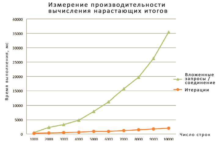
I split the results into two graphs because the nested query or join method is so slow that I had to use a different scale for it. In any case, note that most solutions show a linear relationship between the amount of work and the size of the partition, and only the solution based on a nested query or join shows a quadratic relationship. It is also clear how much more efficient the new solution based on the windowed aggregation function is. The UPDATE-based solution with variables is also very fast, but for the reasons already described, I don't recommend using it. The CLR solution is also quite fast, but it requires you to write all this .NET code and deploy the assembly to the database. No matter how you look at it, the set-based solution using window aggregates remains the preferred solution.