The logical IF operator in Excel is used to write certain conditions. Numbers and/or text, functions, formulas, etc. are matched. When the values meet the specified parameters, one entry appears. Do not answer - another.
Logic functions are a very simple and effective tool that is often used in practice. Let's look at examples in detail.
Syntax of the IF function with one condition
The operator syntax in Excel is the structure of the function, the data necessary for its operation.
IF (logical_expression, value_if_true, value_if_false)
Let's analyze the syntax of the function:
Boolean_expression– WHAT the operator checks (text or numeric cell data).
value_if_true– WHAT will appear in the cell when the text or number meets the specified condition (true).
value if_false– WHAT will appear in the column when the text or number does NOT meet the specified condition (false).
Example:
The operator checks cell A1 and compares it with 20. This is a "logical_expression". When the contents of the column are greater than 20, the true inscription "greater than 20" appears. No - "less than or equal to 20".
Attention! Words in the formula must be enclosed in quotation marks. So that Excel understands that you need to display text values.
One more example. To be admitted to the exam, the students of the group must successfully pass the test. We will put the results in a table with columns: list of students, credits, exam.

Please note: the IF operator must check not the numeric data type, but the text one. Therefore, we wrote in the formula B2 \u003d “credit”. We take quotes so that the program correctly recognizes the text.
IF function in Excel with multiple conditions
Often in practice, one condition for a logical function is not enough. When it is necessary to take into account several options for making decisions, we lay out the IF statements in each other. Thus, we get several IF functions in Excel.
The syntax will look like this:
IF(logical_expression, value_if_true, IF(logical_expression, value_if_true, value_if_false))
Here the operator checks two parameters. If the first condition is true, then the formula returns the first argument, which is true. False - The operator checks the second condition.
Examples of multiple conditions of the IF function in Excel:

Table for performance analysis. The student received 5 points - "excellent". 4 - "good". 3 - "satisfactory". The IF operator checks 2 conditions: the value in cell 5 and 4 are equal.

Expanding functionality with AND and OR operators
When you need to check several true conditions, the AND function is used. The essence is this: IF a \u003d 1 AND a \u003d 2 THEN value in ELSE value c.
The OR function tests condition 1 or condition 2. As soon as at least one condition is true, then the result will be true. The gist is this: IF a = 1 OR a = 2 THEN value in ELSE value c.
The AND and OR functions can test up to 30 conditions.
An example of using the AND operator:
An example of using the OR function:
How to compare data in two tables
Users often need to compare two tables in Excel for matches. Examples from "life": compare the prices of goods in different shipments, compare balance sheets (accounting reports) for several months, the performance of pupils (students) of different classes, in different quarters, etc.
To compare 2 tables in Excel, you can use the COUNTIF operator. Consider the order of application of the function.
For example, let's take two tables with the technical characteristics of different food processors. We conceived highlighting differences with color. Conditional formatting solves this problem in Excel.
Initial data (tables with which we will work):

Select the first table. Conditional formatting - create a rule - use a formula to determine the cells to be formatted:

In the formula bar we write: = COUNTIF (range to compare; first cell of the first table) = 0. The range being compared is the second table.

To drive a range into the formula, simply select its first cell and the last one. "= 0" means a command to search for exact (rather than approximate) values.
We select the format and set how the cells will change when the formula is followed. It is better to fill with color.
Select the second table. Conditional formatting - create a rule - use a formula. We use the same operator (COUNTIF).

Here, instead of the first and last cell of the range, we inserted the column name that we assigned to it in advance. You can fill in the formula in any of the ways. But the name is easier.
Excel. Using worksheet functions. Arguments. Function Wizard. Logical, informational, reference and array functions
 Using Worksheet Functions An Excel function is a special, predefined formula that operates on one or more values and returns a result.
 All functions can be divided into the following groups: l l l -mathematical, -statistical, -logical, -date and time, -financial, -textual, -links and arrays, -database operations, -property and value checks -engineering, -informational
 Function Wizard. Step 1 and 2 l Inserting a function by clicking the function icon on the toolbar l Selecting a function
 Function Wizard. Steps 3 and 4 l l Function Arguments Dialog Box The final step in the Function Wizard. Formula derivation
 Logic Functions Logic functions are integral components of many formulas. They are used whenever it is necessary to perform certain actions depending on the fulfillment of any conditions.

Src="http://present5.com/presentation/3/88838539_293880995.pdf-img/88838539_293880995.pdf-8.jpg" alt="(!LANG:FUNCTION IF Syntax: =IF(logical_expression; value_if_true; value_if_false) l Example: =IF(A 1>3; 10; 20) =IF(B 5>100;"> Функция ЕСЛИ Синтаксис: =ЕСЛИ(логическое_выражение; значение_если_истина; значение_если_ложь) l Пример: =ЕСЛИ(А 1>3; 10; 20) =ЕСЛИ(В 5>100; “Принять”; ”Отказать”) l!}
 Functions AND, OR, NOT l l l Functions AND (AND), OR (OR), NOT (NOT) - allow you to create complex logical expressions. These functions work in conjunction with simple comparison operators. The AND and OR functions can have up to 30 Boolean arguments. Syntax: =AND(boolean 1; boolean 2. . .) =OR(boolean 1; boolean 2. . .) =NOT(boolean)
Src="http://present5.com/presentation/3/88838539_293880995.pdf-img/88838539_293880995.pdf-10.jpg" alt="(!LANG:Functions AND, OR, NOT l Examples: l =IF(AND (A 3>0; D 3>0); “There is a solution”; “Solutions"> Функции И, ИЛИ, НЕ l Примеры: l =ЕСЛИ(И(А 3>0; D 3>0); “Решение есть”; “Решения нет”)) l =ЕСЛИ(ИЛИ(А 3!}


 Nested IF Functions When solving difficult logical problems, you can use nested IF functions l Example: =IF(B 10=25, “Excellent”, IF(AND(B 10 22), “Good”, IF(AND(B 1019), “ Satisfactory”; “Unsatisfactory”))) l
 TRUE and FALSE Functions The TRUE and FALSE functions provide an alternative way to write the logical values TRUE and FALSE. These functions take no arguments and look like this: l =TRUE() l =FALSE() l Example: =IF(A 1=TRUE(); "Go", "Stop") l
Hello, friends! This is an introductory article about Excel functions, where I will explain what functions are, function arguments, how to insert a function into a formula. And in the following posts we will understand what Excel functions are and how to use them correctly.
Functions in Excel are instructions that perform more complex calculations than mathematical operators.. Some calculations cannot be done without functions, so knowing them perfectly is the key to your success.
You can "nest" one function into another, copy formulas with functions (don't forget about ). The main thing is to clearly understand how the function works, otherwise it may give an incorrect result or . You may not even notice it. And to understand how the functions work, read my posts about various functions and Microsoft help.
With the advent of each new version of Excel, the list of functions is updated. Developers add new, popular ones, remove functions that are no longer relevant. In this blog, I will describe the features of Microsoft Excel 2013, but I will answer all questions about features in other versions of the program. As always, ask them in the comments.
Excel Function Arguments
Function Arguments is the initial data for calculating the function. For example, for the SUM (summation) function, this is a list of numbers, cells, or ranges of cells to be summed. Arguments are specified in brackets after the function name and are separated by a semicolon (comma in the English version). By the number of arguments, functions can be:
- no arguments– do not need arguments for calculation. For example, =PI() returns the number 3.1428.
- With one argument- you need to enter only one argument. For example =LOWER(A1) - will convert all characters in the cell to lowercase A1.
- With multiple arguments– you need to enter a certain number of arguments, more than one. For example, the function =MID(A1;1;10) will return the first 10 characters from the string in the cell A1.
- With optional arguments- the function has arguments that are optional. For instance, = VLOOKUP("Ivanov", A1: B30, 2, 0) will look for the last name "Ivanov" in the range A1:B30 and return information about it. The final argument here is "Interval View"- indicates the search method, it is optional to specify.
- With a variable number of arguments– the number of arguments can be changed. For instance, =AVERAGE(A1,B3:B15,C2:F2)– will calculate the average value of the digits in the specified ranges. By listing cells separated by semicolons, you can specify a different number of arguments.
How to insert a function in Excel
To insert a function into a formula, you can use one of the following methods:

If you don't know the function name, use the Insert function window. To call it, try one of the following methods:

After performing any of these operations, the Insert Function window will open. In the Search function box, briefly describe what you need to do and click Find . In field Select function search results will appear. Click on the functions in the list, read their descriptions. If a suitable function is not found, rephrase the query and repeat the search.
When you have found the function, double click on it, the arguments window will open. After filling them in, click OK, the program will calculate the result.
 Window "Function Arguments"
 Again, I state that we have learned an important and simple topic. Still simple! Practice inserting functions into your worksheet yourself and see if it's easy. However, these are very important skills. Their successful application, brought to automatism, is the basis of the foundations. Next, I will describe the work based on the practice of this article.
That's all about inserting functions into a sheet, and in the next article we will start looking at . See you on the blog pages!
Working with large formulas can be problematic even for experienced users. The most difficult thing is to understand someone else's design and understand how it works. Recently, as part of a training, I was asked to parse several complex formulas, and it turned out that the formulas are really rewarded - I counted 7-8 IFs and about 5-6 other functions in one cell. In such situations, it is very important to determine what is the argument of each function. Therefore, I decided to write a short article about an important thing - the Excel argument and its role in calculations. And most importantly, I will describe in the article - how convenient it is to find and highlight each of the arguments when writing huge formulas.
I think you need to first say a few words of banal theory.
Excel argument. Theory
Arguments are the quantities used in the calculation of functions/formulas. Arguments can be a number, text, and even a formula with other functions.
Arguments can be either required (without which the formula will not work) or optional (without which the function will work by default), such are highlighted in square brackets.
DAYWEEK(date_in_number_format;)
Where "date_in_numeric_format" must be filled in, and - can be omitted, and even a semicolon is optional.
It is important to note that functions may not contain an argument.
TODAY()
Or they can be with a non-constant number of arguments, like:
SUMIFS()
How to conveniently find and highlight function arguments?
To understand large, heavy formulas, it is very important to be able to highlight the arguments of nested functions. Even if you have written this formula, I guarantee you that in six months you will not understand it right away. To conveniently see the function argument, click on the tooltip below, which will appear when entering the cell and the argument will be highlighted:
In the example, click on the “search value” and in the formula itself it will be highlighted with a highlight.
For convenience, I also attach a gif
But there are records and heavier. Such:
Or such
The formulas are not mine, I hope the creators will not be offended. I am sure many (including myself) have met mountains of symbols and more serious ones. It is extremely difficult to understand such constructions without the possibility of selection.
What else is important to say
With such constructions, it is very important to understand the formula in parts, to highlight its argument. Excel's argument selection method is very handy. I can also advise to spread each function on a new line with Alt + Enter - it also helps a lot - more details here.
It is also important to note that the selection of a function argument can be done after the selection of any argument of the formula.
For example, it is not clear to you how the function in the example works (I did not specifically fill in the 4th argument of the VLOOKUP).
You can click on any place in the formula with the mouse, after which a hint will appear for you which argument it is.
From this hint, you can jump to any of the arguments by clicking on it.
And you can also go to the help by clicking on the name of the formula itself, in this case VLOOKUP.
Successful analysis of your own and other people's formulas! Write your comments.
(Visited 523 times, 1 visits today)
Hello, friends! This is an introductory article about Excel functions, where I will explain what functions are, function arguments, how to insert a function into a formula. And in the following posts we will understand what Excel functions are and how to use them correctly.
Functions in Excel are instructions that perform more complex calculations than mathematical operators.. Some calculations cannot be done without functions, so their perfect knowledge is the key to your success.
You can "nest" one function into another, copy formulas with functions (don't forget about different types of links). The main thing is to clearly understand how the function works, otherwise it may give an incorrect result or an error. You may not even notice it. And to understand how the functions work, read my posts about various functions and Microsoft help.
With the advent of each new version of Excel, the list of functions is updated. Developers add new, popular ones, remove functions that are no longer relevant. In this blog, I will describe the features of Microsoft Excel 2013, but I will answer all questions about features in other versions of the program. As always, ask them in the comments.
Excel Function Arguments
Function Arguments is the initial data for calculating the function. For example, for the SUM (summation) function, this is a list of numbers, cells, or ranges of cells to be summed. Arguments are specified in brackets after the function name and are separated by a semicolon (in the English version - a comma). By the number of arguments, functions can be:
- no arguments– do not need arguments for calculation. For example, =PI() returns the number 3.1428.
- With one argument- you need to enter only one argument. For example =LOWER(A1) - will convert all characters in cell A1 to lowercase.
- With multiple arguments– you need to enter a certain number of arguments, more than one. For example, the function =MID(A1;1;10) will return the first 10 characters from the string in cell A1.
- With optional arguments- the function has arguments that are optional. For example, =VLOOKUP(“Ivanov”, A1:B30,2,0) will search for the last name “Ivanov” in the range A1:B30 and return information about him. The last argument here - "Interval lookup" - indicates the search method, it is optional to specify it.
- With a variable number of arguments– the number of arguments can be changed. For example, =AVERAGE(A1;B3:B15;C2:F2) - will calculate the average value of the digits in the specified ranges. By listing cells separated by semicolons, you can specify a different number of arguments.
How to insert a function in Excel
To insert a function into a formula, you can use one of the following methods:

If you don't know the function name, use the Insert function window. To call it, try one of the following methods:

After performing any of these operations, the Insert Function window will open. In the Search function field, briefly describe what you need to do and click Search. The search results appear in the Select a function box. Click on the functions in the list, read their descriptions. If a suitable function is not found, rephrase the query and repeat the search.
When you have found the function, double click on it, the arguments window will open. After filling them, click OK, the program will calculate the result.
 Window "Function Arguments"
Again, I state that we have learned an important and simple topic. Still simple! Practice inserting functions into your worksheet yourself and see if it's easy. However, these are very important skills. Their successful application, brought to automatism, is the basis of the foundations. Next, I will describe the work based on the practice of this article.
That's all about inserting functions into a sheet, and in the next article we will start looking at text functions. See you on the OfficeEASY.com blog pages!
Excel contains many built-in functions that can be used for engineering, statistical, financial, analytical and other calculations. Sometimes the conditions of the tasks set require a more flexible tool for finding a solution, then macros and user-defined functions come to the rescue.
An example of creating your own custom function in Excel
Like macros, user-defined functions can be created using the VBA language. To implement this task, you must perform the following steps:
- Open the VBA language editor using the ALT+F11 key combination.
- In the window that opens, select the Insert item and the Module sub-item, as shown in the figure:
- A new module will be created automatically, and a window for entering code will appear in the main part of the editor window:
- If necessary, you can change the name of the module.
- Unlike macros, whose code must be between the Sub and End Sub statements, user-defined functions are denoted by the Function and End Function statements, respectively. The user-defined function includes a name (an arbitrary name that reflects its essence), a list of parameters (arguments) with a declaration of their types, if required (some may not accept arguments), a return type, a function body (code that reflects the logic of its work) , as well as the End Function statement. An example of a simple user-defined function that returns the names of the day of the week, depending on the specified number, is shown in the figure below:
- After entering the above code, you must press the key combination Ctrl + S or a special icon in the upper left corner of the code editor to save.
- To use the created function, you need to return to the Excel spreadsheet editor, place the cursor in any cell and enter the name of the custom function after the “=” symbol:
Built-in Excel functions contain explanations of both the result they return and the arguments they take. This can be seen on the example of any function by pressing the SHIFT + F3 hot key combination. But our function doesn't have a form yet.
To document a custom function, you need to do the following:
- Create a new macro (press the key combination Alt+F8), in the window that appears, enter an arbitrary name for the new macro, click the Create button:
- As a result, a new module will be created with a blank, limited by the Sub and End Sub statements.
- Enter the code as shown in the figure below, specifying the required number of variables (depending on the number of arguments to the user-defined function):
- A text string with the name of the custom function should be passed as "Macro", as "Description" - a String type variable with a description text of the returned value, as "ArgumentDescriptions" - an array of String type variables with description texts of the custom function arguments.
- To create a description of a user-defined function, it is enough to execute the module created above once. Now, when calling a user-defined function (or SHIFT+F3), a description of the returned result and variable is displayed:
Function descriptions are optional. They are necessary in cases where user-defined functions will be used frequently by other users.
Examples of using user-defined functions that are not in Excel
View of the original data table:
Each employee is entitled to 24 days off with payment S=N*24/(365-n), where:
- N is the total salary for the year;
- n is the number of holidays in a year.
Let's create a custom function for calculation based on this formula:
Example code:
Public Function Otpusknye(summZp As Long, holidays As Long) As Long
If IsNumeric(holidays) = False Or IsNumeric(summZp) = False Then
Otpusknye = "Non-numeric data entered"
exit function
ElseIf holidays
Functions represent the dependence of one element (result) on other elements (arguments, .. those inside :-)). It's kind of understandable. In order to use any function in Excel, you must enter it as a formula (the nuances are described here) or as part of a formula into a worksheet cell. The sequence in which the symbols and arguments used in the formula must be located is called the syntax of the function. All functions use the same syntax rules. If you violate these rules, then Excel will display a message stating that there is an error in the formula and will not be friends with you. But believe me, everything is quite the same in Excel functions, and having understood once, on one or two functions, in other cases everything will be quite simple. Syntax rules for writing functions The following are the rules that must be followed for the competent and optimal construction of a formula using one or more functions. If a function appears at the very beginning of a formula, it must be preceded by an equal sign, as is the case at the beginning of any formula. I have already spoken about this in previous articles but it's not a sin to repeat. After that, the name of the function is entered, followed immediately by the list of arguments in parentheses. Arguments are separated from each other by a semicolon ";". The parentheses allow Excel to determine where the argument list starts and ends.Excel function Note that the function entry must contain opening and closing brackets, and you cannot insert spaces between the function name and the brackets. Otherwise, Excel will issue an error message. You can use numbers, text, booleans, arrays, error values, or references as arguments. In this case, the parameters specified by the user must have valid values for this argument. For example, the formula below sums the values in cells B2, B3, B4, B5, and E7, with some of the cells, B2 to B5, being represented as a continuous range.
Excel function arguments Let's consider the work of the ROUND(arg1;arg2) function, which returns a number rounded to a specified number of decimal places, and has two arguments: arg1 - the address of the cell with the number (or the number itself) to be rounded; arg2 - the number of digits after the decimal point in the number after rounding.
To round the number 2.71828 in cell A1 to one, two, or three decimal places and write the calculation results to cells B1, C1, and D1, respectively, proceed as follows. Enter the number 2.71828 in cell A1. Enter the following formulas into cells B1, C1 and D1: =ROUND(A1;1) =ROUND(A1;2) =ROUND(A1;3) Arguments can be either constants or functions. Functions that are arguments to another function are called nested functions. For example, let's sum the values of cells A1 and A2, after rounding these values to two decimal places: =SUM(ROUND(A1;2);Round(A2;2)) Excel formulas can be used up to seven nesting levels functions. It is worth noting that there are functions in Excel that do not take arguments. Examples of such functions are PI (returns the value of π rounded to 15 digits) or TODAY (returns the current date). When using such functions, you should put empty parentheses without arguments in the formula bar immediately after the function name. In other words, to get the value of the number p or the current date in the cells, you should enter formulas of the following form: =PI() =TODAY() lists, date and time functions, financial, statistical, textual, mathematical, logical. Text functions are used for text processing, namely: searching for the desired characters, writing characters to a strictly defined place in the text, etc. Using the Date and Time functions, you can solve almost any task related to calendar dates or times (for example, calculate the number of working days for any period of time). Boolean functions are used to create complex formulas that, depending on the fulfillment of certain conditions, will implement various types of data processing. They are especially interesting, and we will talk about them in a separate article. Mathematical functions are widely represented in Excel, and I have already given some of them in examples. The user also has at his disposal a library of Statistical functions, with which you can search for the average value, maximum and minimum elements, etc.
Arguments is information that the function uses to calculate a new value or perform an action. Arguments are always to the right of the function name and enclosed in parentheses. Most arguments are of a specific type. In fact, the argument being given must either be of a suitable type, or one that Microsoft Excel can convert to a suitable type.
Function arguments can be numeric values, cell references, ranges, names, text strings, and nested functions.
When an argument is followed by an ellipsis (...) when describing the syntax of a function, it means that there can be more than one argument of the same type. Some functions can have up to 30 arguments, as long as the total number of characters in the formula does not exceed 1024. For example, the syntax for the MAX function is as follows:
MAX(number1, number2, ...)
Any of the following formulas are valid:
MAX(26;31;29)
Functions with an empty pair of parentheses after their name require no arguments, but you must include these empty parentheses in the formula for Microsoft Excel to recognize the function.
Many argument names in a function's syntax description hint at what information should be given as the actual value of the argument. For example, for the function ROUND(number; number_of_digits), the first argument must be a number and the second must also be a number.
Likewise, words such as number, reference, flag, text, array, when used as an argument name, indicate that the argument must be of the appropriate type. Word Meaning implies that the argument can be anything that is a single value. That is, the value can be a number, text, a Boolean value, or an error value.
Using Arguments
The argument can be anything that delivers a value of the required type. For example, a SUM function that sums its arguments can take anywhere from 1 to 30 arguments. The SUM functions can be passed any of the following four kinds of arguments, as long as they deliver a number or numbers:
– a value that is a number, for example: SUM(1;10;100);
is a formula that results in a number, for example: SUM(0.5+0.5;AVERAGE(5;5);10^2). Functions that are used as arguments to other functions, as in the previous example, are called nested functions. In this example, the function AVERAGE is a function argument SUM. The level of nesting of functions in formulas can be up to seven;
SUM(A1;A2)
SUM(A1:A5)
The second example is equivalent to the formula SUM(A1,A2,A3,A4,A5). The advantage of using an interval is that the argument A1:A5 counts as one argument, while A1, A2, A3, A4, A5 count as five arguments. If you need to add more than 30 numbers, then you will have to use intervals, because the function cannot have more than 30 arguments;
– a name that refers to a value, formula, cell, or range of cells containing numbers or formulas that deliver numbers, for example: SUM(Base; Increment).
Argument types. Function arguments can be any of the following objects.
Numbers. Examples of numbers are 5.003, 0, 150.286, and -30.05. Numbers without a decimal point are called integers. Examples of integers are 5, 0, 150, and -30. Numbers can have up to 15 significant digits.
Text. Examples of texts are "a", "Word", "sign/punctuation", and "" (empty text). Text values used in formulas must be enclosed in double quotes. If the text itself contains double quotes, then they should be doubled. For example, to determine the length (in characters) of "in the 'good' old time" text, you could use the formula:
DLSTR("in the""good""old times")
Text values can be up to 32000 characters long, including double quotes. A text constant that contains no characters is written as "" and is called "blank text".
Note . If the text used as an argument is not enclosed in double quotes, then Microsoft Excel assumes that it is a name and tries to substitute the value that the name refers to instead. If the unquoted text is not a name, and therefore has no value, Microsoft Excel will return an error value #NAME?.
Boolean values. Boolean values are TRUE and FALSE. Boolean arguments can also be expressions, such as B10>20, whose values are TRUE or FALSE.
Error values. The error values are #DIV/0!, #N/A, #NAME?, #BLANK!, #NUMBER!, #LINK! and #VALUE!.
Links. Examples of links are $A$10, A10, $A10, A$10, R1C1 or RC[-10]. Links can point to single cells, cell ranges, or multiple cell selections, and can be relative, absolute, or mixed. If a link is used as an argument, which must be a number, text, boolean, or error value, then the contents of the cell identified by the link is used as the actual argument.
SUM((E5:E8;E10:E18); AVERAGE(A1:A5))
Arrays. Arrays allow you to control how arguments and functions are entered into cells. Using arrays simplifies the development of some worksheet formulas and saves memory. Microsoft Excel defines two types of arrays: array ranges and constant ranges. An array range is a contiguous range of cells that share a common formula; a range of constants is a set of constants used as arguments to functions.
Using semicolons in argument list
Individual arguments must be separated by semicolons, but there must be no extra semicolons. If a semicolon is used only to mark the location of an argument, and the argument itself is not specified, then Microsoft Excel substitutes the default value for that argument, unless the argument is required. For example, if you enter (;arg2;arg3) as the argument list for a function with three arguments, Microsoft Excel will substitute the appropriate value for arg1. If you enter (arg1;;), the appropriate values will be substituted for arg2 and arg3.
For those functions that count the number of arguments before evaluation, the extra semicolons will count towards the number of arguments and will therefore affect how the function's value is calculated. For instance, AVERAGE(1;2;3;4;5) is 3, but AVERAGE(;;1;2;3;4;5) equals 2.14.
For most arguments, the value substituted for the omitted argument is 0, FALSE, or "" (empty text), depending on what the type of the argument should be. For an omitted reference argument, the default value is usually the active cell or selection.