James Loy, Georgia Tech. A beginner's guide, after which you can create your own neural network in Python.
Motivation:based on my personal experience in learning deep learning, I decided to create a neural network from scratch without a complex learning library such as. I believe that understanding the internal structure of a neural network is important for a beginner Data Scientist.
This article contains what I have learned and hopefully it will be useful for you too! Other helpful related articles:
What is a neural network?
Most articles on neural networks draw parallels with the brain when describing them. It's easier for me to describe neural networks as a mathematical function that maps a given input to a desired output without going into details.
Neural networks are composed of the following components:
- input layer, x
- arbitrary amount hidden layers
- output layer, ŷ
- set scales and displacements between each layer W and b
- choice activation functions for each hidden layer σ ; in this work we will use the activation function of Sigmoid
The diagram below shows the architecture of a two-layer neural network (note that the input layer is usually excluded when counting the number of layers in the neural network).
Creating a Neural Network class in Python looks simple:
Neural network training
Output ŷ a simple two-layer neural network:
In the above equation, the weights W and bias b are the only variables that affect the output ŷ.
Naturally, the correct values \u200b\u200bfor the weights and biases determine the accuracy of the predictions. The process of fine-tuning weights and biases from input data is known as neural network training.
Each iteration of the training process consists of the following steps
- calculating the predicted output ŷ called forward propagation
- updating weights and biases called backpropagation
The sequential graph below illustrates the process:
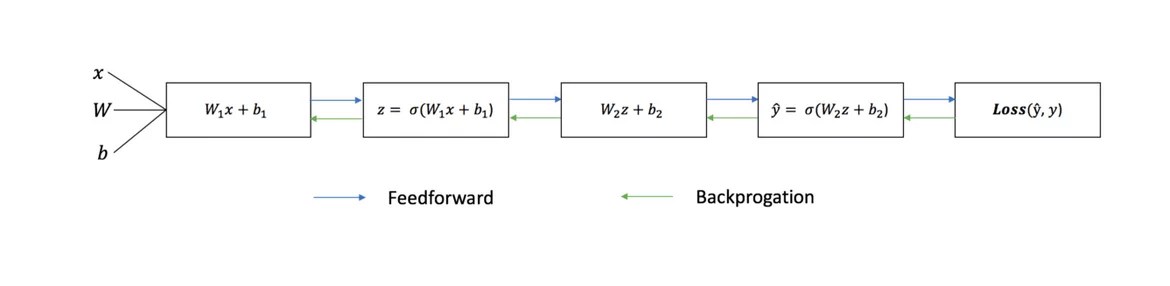
Direct distribution
As we saw in the graph above, forward propagation is just a simple computation, and for a basic 2-layer neural network, the output of the neural network is given by:
Let's add feed forward to our Python code to do this. Note that for simplicity, we have assumed that the offsets are 0.
However, we need a way to assess the "goodness" of our forecasts, that is, how far our forecasts are). Loss function just allows us to do it.
Loss function
There are many loss functions available, and the nature of our problem should dictate our choice of loss function. In this work we will use sum of squares of errors as a loss function.

The sum of squared errors is the average of the difference between each predicted value and the actual value.
The goal of training is to find a set of weights and biases that minimizes the loss function.
Back propagation
Now that we have measured our forecast error (loss), we need to find a way propagating the error back and update our weights and biases.
To know the appropriate sum to correct for weights and biases, we need to know the derivative of the loss function with respect to the weights and biases.
Recall from the analysis that the derivative of the function is the slope of the function.

If we have a derivative, then we can simply update the weights and biases by increasing / decreasing them (see diagram above). It is called gradient descent.
However, we cannot directly calculate the derivative of the loss function with respect to the weights and biases, since the equation of the loss function does not contain weights and biases. Therefore, we need a chain rule to help us calculate.
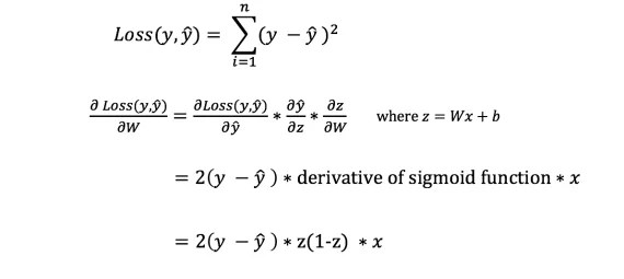
Fuh! It was cumbersome, but it allowed us to get what we need - the derivative (slope) of the loss function with respect to the weights. We can now adjust the weights accordingly.
Let's add the backpropagation function to our Python code:
Checking the operation of the neural network
Now that we have our complete Python code for doing forward and backpropagation, let's take a look at our neural network by example and see how it works.
 The perfect set of weights
 Our neural network needs to learn the ideal set of weights to represent this function.
Let's train a neural network for 1500 iterations and see what happens. Looking at the iteration loss graph below, we can clearly see that the loss monotonically decreases to a minimum. This is consistent with the gradient descent algorithm we talked about earlier.

Let's look at the final prediction (output) from the neural network after 1500 iterations.

We did it!Our forward and backward propagation algorithm has shown the neural network to work well, and the predictions converge on true values.
Note that there is little difference between the predictions and the actual values. This is desirable because it prevents overfitting and allows the neural network to better generalize invisible data.
Final reflections
I learned a lot in the process of writing my own neural network from scratch. While deep learning libraries such as TensorFlow and Keras allow deep networks to be built without fully understanding the inner workings of a neural network, I find it helpful for aspiring Data Scientists to gain a deeper understanding of them.
I have invested a lot of my personal time in this work, and I hope you find it useful!
This week you could read an extremely motivating case from a GeekBrains student who studied the profession, where he talked about one of his goals, which led to the profession - the desire to learn the principle of work and learn how to create game bots yourself.
Indeed, it was the desire to create perfect artificial intelligence, be it a game model or a mobile program, that prompted many of us to the path of a programmer. The problem is that, behind tons of educational material and the harsh reality of customers, this very desire has been replaced by a simple desire for self-development. For those who have not yet begun to fulfill their childhood dreams, here is a short guide to creating a real artificial intelligence.
Stage 1. Disappointment
When we talk about creating at least simple bots, the eyes are filled with sparkle, and hundreds of ideas flash in his head about what he should be able to do. However, when it comes to implementation, it turns out that mathematics is the key to unraveling the actual behavior. Yes, artificial intelligence is much more difficult than writing application programs - knowledge about software design alone will not be enough for you.
Mathematics is the scientific springboard on which your further programming will be built. Without knowledge and understanding of this theory, all ideas will quickly break up about interaction with a person, because an artificial mind is really nothing more than a set of formulas.
Stage 2. Acceptance
When the arrogance is a little knocked down by student literature, you can start practice. Throwing yourself into LISP or others is not worth it yet - you should first get comfortable with the principles of AI design. Python is perfect for both quick learning and further development - this is the language most often used for scientific purposes, for it you will find many libraries that will make your work easier.
Stage 3. Development
Now we turn directly to the theory of AI. They can be roughly divided into 3 categories:
- Weak AI - bots that we see in computer games, or simple helpers like Siri. They either perform highly specialized tasks or are an insignificant complex of them, and any unpredictability of interaction baffles them.
- Strong AIs are machines whose intelligence is comparable to the human brain. Today, there are no real representatives of this class, but computers like the Watson are very close to achieving this goal.
- Perfect AI is the future, a machine brain that will surpass our capabilities. It is about the dangers of such developments that Stephen Hawking, Elon Musk and the Terminator film franchise warn.
Naturally, you should start with the simplest bots. To do this, remember the good old tic-tac-toe game when using the 3x3 field and try to figure out the basic algorithms for yourself: the probability of winning with error-free actions, the most successful places on the field for a piece, the need to reduce the game to a draw, and so on.
Several dozen games and analyzing your own actions, you can probably highlight all the important aspects and rewrite them into machine code. If not, keep thinking, and this link is here just in case.
By the way, if you still took up the Python language, then you can create a fairly simple bot by referring to this detailed manual. For other languages, such as C ++ or Java, you won't have any trouble finding step-by-step materials either. Feeling that there is nothing supernatural behind the creation of AI, you can safely close the browser and start personal experiments.
Stage 4. Excitement
Now that things have gotten off the ground, you probably want to create something more serious. A number of the following resources will help you with this:
As you understand even from the names, these are APIs that will allow you to create some semblance of serious AI without wasting time.
Stage 5. Work
Now, when you already quite clearly understand how to create AI and what to use at the same time, it's time to take your knowledge to a new level. First, it will require a discipline study called "Machine Learning". Secondly, you need to learn how to work with the appropriate libraries of the selected programming language. For the Python we are considering, these are Scikit-learn, NLTK, SciPy, PyBrain, and Numpy. Thirdly, development is indispensable. And most importantly, you will now be able to read AI literature with full understanding of the matter:
- Artificial Intelligence for Games, Ian Millington;
- Game Programming Patterns, Robert Nystorm;
- AI Algorithms, Data Structures, and Idioms in Prolog, Lisp, and Java, George Luger, William Stbalfield;
- Computational Cognitive Neuroscience, Randall O'Reilly, Yuko Munakata;
- Artificial Intelligence: A Modern Approach, Stuart Russell, Peter Norvig.
And yes, all or almost all of the literature on this topic is presented in a foreign language, so if you want to create AI professionally, you need to improve your English to a technical level. However, this is relevant for any area of \u200b\u200bprogramming, isn't it?
We are currently experiencing a real boom in neural networks. They are used for image recognition, localization and processing. Neural networks are already able to do a lot that is not accessible to humans. We must also wedge ourselves into this matter! Consider a neutron network that will recognize numbers in the input image. It's very simple: just one layer and an activation function. This will not allow us to recognize absolutely all test images, but we will cope with the vast majority. As data, we will use the MNIST data collection known in the world of number recognition.
There is a python-mnist library for working with it in Python. To install:
Pip install python-mnist
Now we can load data
From mnist import MNIST mndata \u003d MNIST ("/ path_to_mnist_data_folder /") tr_images, tr_labels \u003d mndata.load_training () test_images, test_labels \u003d mndata.load_testing ()
The archives with the data must be loaded independently, and the program must specify the path to the directory with them. Now the variables tr_images and test_images contain images for network training and testing, respectively. And the variables tr_labels and test_labels are labels with the correct classification (i.e. numbers from images). All images are 28x28. Let's set a variable with a size.
Img_shape \u003d (28, 28)
Let's convert all the data to numpy arrays and normalize them (we will bring them to the size from -1 to 1). This will increase the accuracy of the calculations.
Import numpy as np for i in range (0, len (test_images)): test_images [i] \u003d np.array (test_images [i]) / 255 for i in range (0, len (tr_images)): tr_images [i] \u003d np.array (tr_images [i]) / 255
I note that although it is customary to represent images as a two-dimensional array, we will use a one-dimensional array, it is easier for calculations. Now you need to understand "what is a neural network"! And this is just an equation with a lot of coefficients. We have at the input an array of 28 * 28 \u003d 784 elements and 784 more weights to determine each digit. During the operation of the neural network, you need to multiply the values \u200b\u200bof the inputs by the weights. Add up the received data and add an offset. Submit the result to the activation function. In our case, it will be Relu. This function is zero for all negative arguments and an argument for all positive ones.

There are many more activation functions! But this is the simplest neural network! Let's define this function using numpy
Def relu (x): return np.maximum (x, 0)
Now, to calculate the image in the picture, you need to calculate the result for 10 sets of coefficients.
Def nn_calculate (img): resp \u003d list (range (0, 10)) for i in range (0,10): r \u003d w [:, i] * img r \u003d relu (np.sum (r) + b [ i]) resp [i] \u003d r return np.argmax (resp)
For each set, we will get an output. The output with the highest score is most likely our number.

In this case, 7. That's it! But no ... After all, you need to take these same coefficients somewhere. We need to train our neural network. For this, the backpropagation method is used. Its essence is to calculate the outputs of the network, compare them with the correct ones, and then subtract from the coefficients the numbers necessary for the result to be correct. It should be remembered that in order to calculate these values, the derivative of the activation function is needed. In our case, it is zero for all negative numbers and 1 for all positive ones. Let's determine the coefficients in a random way.
W \u003d (2 * np.random.rand (10, 784) - 1) / 10 b \u003d (2 * np.random.rand (10) - 1) / 10 for n in range (len (tr_images)): img \u003d tr_images [n] cls \u003d tr_labels [n] #forward propagation resp \u003d np.zeros (10, dtype \u003d np.float32) for i in range (0,10): r \u003d w [i] * img r \u003d relu ( np.sum (r) + b [i]) resp [i] \u003d r resp_cls \u003d np.argmax (resp) resp \u003d np.zeros (10, dtype \u003d np.float32) resp \u003d 1.0 #back propagation true_resp \u003d np. zeros (10, dtype \u003d np.float32) true_resp \u003d 1.0 error \u003d resp - true_resp delta \u003d error * ((resp\u003e \u003d 0) * np.ones (10)) for i in range (0,10): w [i ] - \u003d np.dot (img, delta [i]) b [i] - \u003d delta [i]
In the process of training, the coefficients will become slightly similar to numbers:
Let's check the accuracy of the work:
Def nn_calculate (img): resp \u003d list (range (0, 10)) for i in range (0,10): r \u003d w [i] * img r \u003d np.maximum (np.sum (r) + b [ i], 0) #relu resp [i] \u003d r return np.argmax (resp) total \u003d len (test_images) valid \u003d 0 invalid \u003d for i in range (0, total): img \u003d test_images [i] predicted \u003d nn_calculate (img) true \u003d test_labels [i] if predicted \u003d\u003d true: valid \u003d valid + 1 else: invalid.append (("image": img, "predicted": predicted, "true": true)) print ("accuracy () ". format (valid / total))
I got 88%. Not so cool, but very interesting!
This time, I decided to study neural networks. I was able to get basic skills in this matter over the summer and fall of 2015. By basic skills, I mean I can build a simple neural network myself from scratch. You can find examples in my repositories on GitHub. In this article, I will provide some clarification and share resources that you may find useful to explore.
Step 1. Neurons and the feedforward method
So what is a "neural network"? Let's wait with that and deal with one neuron first.
A neuron is like a function: it takes several values \u200b\u200bas input and returns one.
The circle below represents an artificial neuron. It gets 5 and returns 1. Input is the sum of the three synapses connected to the neuron (three arrows on the left).
On the left side of the picture, we see 2 input values \u200b\u200b(green) and an offset (highlighted in brown).
The input data can be numerical representations of two different properties. For example, when creating a spam filter, they could mean the presence of more than one word in CAPITAL LETTERS and the presence of the word "viagra".
The input values \u200b\u200bare multiplied by their so-called "weights", 7 and 3 (highlighted in blue).
Now we add the resulting values \u200b\u200bwith the offset and get a number, in our case 5 (highlighted in red). This is the input of our artificial neuron.

Then the neuron performs some kind of calculation and outputs an output value. We got 1 because the rounded sigmoid value at point 5 is 1 (more on this function later).
If it were a spam filter, the fact of output 1 would mean that the text was marked as spam by the neuron.

Neural network illustration from Wikipedia.
If you combine these neurons, you get a straight-forward neural network - the process goes from input to output, through neurons connected by synapses, as in the picture on the left.
Step 2. Sigmoid
After you've watched the Welch Labs tutorials, it's a good idea to check out the fourth week of Coursera's Machine Learning Neural Networks course to help you understand how they work. The course is very deep in math and is based on Octave, and I prefer Python. Because of this, I skipped the exercises and learned all the necessary knowledge from the video.

The sigmoid simply maps your value (along the horizontal axis) to a range from 0 to 1.
The first priority for me was to study the sigmoid, as it figured in many aspects of neural networks. I already knew something about her from the third week of the above course, so I reviewed the video from there.
But videos alone won't get you very far. For a complete understanding, I decided to code it myself. So I started writing an implementation of a logistic regression algorithm (which uses a sigmoid).
It took a whole day and the result was hardly satisfactory. But it doesn't matter, because I figured out how everything works. You can see the code.
You don't have to do it yourself, since it requires special knowledge - the main thing is that you understand how the sigmoid works.
Step 3. Backpropagation method
It is not so difficult to understand how a neural network works from input to output. It is much more difficult to understand how a neural network is trained on datasets. The principle I used is called