Signal types
Signal
Signal is a physical process, some characteristic of which carries informational meaning.
For example, a light signal (light flux) is characterized by brightness, color, polarization properties, direction of propagation, etc.
Information can be carried either by one of these characteristics or by a simultaneous combination of several characteristics.
The signal occurs in nature during the interaction of material objects and carries information about this interaction. The signal is able to move, propagate in some material environment, thereby providing spatial transfer of information from the object (event source) to the subject (observer). The material medium in which the signal propagates is called signal carrier.
Signals differ primarily in their physical nature. Examples: light signal, sound signal, electrical signal, radio signal...
Depending on the source that generates them, the signals are natural or artificial.
Natural signals arise due to the fact that somewhere in animate or inanimate nature material objects interact. This is a natural process that has nothing to do with human activity. Examples: the glow of the Sun, the singing of birds, the spread of the smell of flowers ...
Artificial signals are initiated by a person or appear in technical systems created by a person. Examples: telephone line electrical signals; radio signals; flare or bonfire; traffic signal; fire truck siren...
The shape of the signals are analog, discrete and digital.
Analog (or continuous) signal is a physical process, the information characteristic of which changes smoothly. For example, a smoothly changing electrical signal (Fig. 1). Other examples: sound signal, natural light signal. Almost all natural signals are analog.
A feature of an analog signal is the blurring of the boundary between its two adjacent values. The total number of values that can characterize an analog signal is infinite.
discrete signal is a physical process, the information characteristic of which changes abruptly and can only take on a certain limited set of values (Fig. 2).
A feature of a discrete signal is a clear distinction between two different signal values. The total number of possible values that a discrete signal can take is always limited.
For example, a lamp connected to an electrical circuit. The lamp may either be on or off. If the lamp is on, this serves as a signal that there is current in the circuit. If it is not lit, there is no current. Intermediate values (with what brightness the lamp burns) are not taken into account here - there are only two values: either on or off.
Another example: a certain message is transmitted by telegraph.
The message is transmitted using Morse code, which uses three different values: dot, dash, and space (pause). The signal that carries this message will also have only three different meanings: short signal, long signal and no signal. Since the number of possible signal values is limited, this is a discrete signal.
Discrete signals are usually artificial(created by a person or a technical system).
1. Basic concepts and definitions. Definition of radio electronics. Definition of radio engineering. The concept of a signal. Classification analysis of signals. Classification analysis of radio circuits. Classification analysis of radio electronic systems.

Modern radio electronics is a generalized name for a number of areas of science and technology related to the transmission and transformation of information based on the use and transformation of electromagnetic oscillations and radio frequency waves; the main of these areas are:
radio engineering, radiophysics and electronics.
The main task of radio engineering is to transmit information over a distance using electromagnetic oscillations. In a broader sense, modern radio engineering is a field of science and technology associated with the generation, amplification, conversion, processing, storage, transmission and reception of radio frequency electromagnetic waves used to transmit information over a distance. As follows from this, radio engineering and radio electronics are closely related and often these terms replace each other.
The science that studies the physical foundations of radio engineering is called radiophysics.
1. The concept of a signal.
A signal (from Latin signum - a sign) is a physical process or phenomenon that carries a message about an event, the state of an object, or transmits control commands, alerts, etc. Thus, the signal is the material carrier of the message. Any physical process (light, electric field, sound vibrations, etc.) can serve as such a carrier. In radio electronics, mainly electrical signals are studied and used. Signals as physical processes are observed using various instruments and devices (oscilloscope, voltmeters, receivers). Any model reflects a limited number of the most significant features of a real physical signal. Insignificant features of the signal are ignored to simplify the mathematical description of the signals. The general requirement for a mathematical model is the maximum approximation to the real process with the minimum complexity of the model. Functions that describe signals can take real and complex values, so they often talk about real and complex signal models.
Signal classification. According to the possibility of predictions inst. signal values at any time are different:
Deterministic signals, i.e. such signals for which instantaneous values for any moment of time are known and predictable with a probability equal to one;
Random signals, i.e. such signals, the value of which at any moment of time cannot be predicted with a probability equal to one.
All signals that carry information are random, since a completely deterministic signal (known) does not contain information.
The simplest examples of deterministic and random signals are mains voltages and noise voltages, respectively (see Figure 2.1).

In turn, random and deterministic signals can be divided into continuous or analog signals and discrete signals, which have several varieties. If the signal can be measured (observed) at any time, then it is called analog. Such a signal exists at any time. Discrete signals can be observed and measured in discrete (separate) time intervals limited in duration by the time they appear. Discrete signals include pulse signals.
The figure shows two types of pulses. Video pulse and radio pulse. When generating radio pulses, the video pulse is used as a control (modulating) signal, and in this case there is an analytical relationship between them: 
In this case, it is called the envelope of the radio pulse, and the function is called its filling.
It is customary to characterize pulses with amplitude A, duration , duration of rise and cut, and, if necessary, frequency or repetition period.
Pulse signals can be of various types. In particular, there are impulse signals called discrete (see Fig. 2.3).
This kind of signals can be represented by a mathematical model as a countable set of function values - where i = 1, 2, 3, ...., k, counted at discrete times. The signal sampling step in time and in amplitude is usually a constant value for a given type of signal, i.e. minimum signal increment
Each of the values of the finite set S can be represented in the binary system as a number: - 10101; - 11001; - 10111. Such signals are called digital.
Classification of radio systems and the tasks they solve
According to the functions performed, radio information systems can be divided into the following classes:
information transmission (radio communication, broadcasting, television);
extracting information (radar, radio navigation, radio astronomy, radio measurements, etc.);
destruction of information (radio countermeasures);
management of various processes and objects (unmanned aerial vehicles, etc.);
combined.
In the information transmission system there is a source of information and its recipient. In a radio system for extracting information, information as such is not transmitted, but is extracted either from own signals emitted towards the object under study and reflected from it, or from signals from other radio systems, or from own radio emission of various objects.
Information destruction radio systems serve to interfere with the normal operation of a competing radio system by emitting an interfering signal, or by receiving, deliberately distorting and re-radiating a signal.
In radio control systems, the task of executing by an object a certain command sent from the control panel is solved. Command signals are information for the tracking device executing the command.
The main tasks solved by the radio system when receiving information are:
Detection of a signal against the background of interference.
Distinguishing signals against the background of interference.
Estimation of signal parameters.
Play message.
The first problem is most simply solved, in which, with given probabilities of correct detection and false alarm, a decision should be made about the presence of a known signal in the received message. The higher the task level, the more complex the circuitry of the receiving device becomes.

2. Energy, power, orthogonality and coherence of signals. Mutual energy of signals (similarity integral). The concept of signal norm.
There are four types of signals s(t): continuous continuous time, continuous discrete time, discrete continuous time and discrete discrete time.
Continuous continuous time signals are referred to as continuous (analog) signals for short. They can change at arbitrary moments, taking on any of a continuous set of possible values (Fig. 1.3). The well-known sinusoid also belongs to such signals.
Rice. 1.3 Continuous signal

Rice. 1.4 Continuous discrete time signal
Continuous signals of discrete time can take arbitrary values, but change only at certain, predetermined (discrete) moments (Fig. 1.4).
Discrete signals of continuous time differ in that they can change at arbitrary times, but their values take only allowed (discrete) values (Fig. 1.5).
Discrete signals of discrete time (abbreviated as discrete) (Fig. 1.6) at specific times can only take allowed (non-specific) values.
The signals generated at the output of the converter of a discrete message into a signal, as a rule, are discrete in terms of the information parameter, i.e., they are described by a function of discrete time and a finite set of possible values. In data transmission engineering, such signals are called digital data signals (DDC). The parameter of the data signal, the change of which reflects the change in the message, is called representing (information). On fig. Figure 1.7 shows a DSD whose representative parameter is amplitude, and the set of possible values of the representative parameter is equal to two. Part of the digital data signal, which differs from the rest of the parts by the value of one of its representing ones. parameters is called the DAC element.
The fixed value of the state representing the parameter of the signal is called the significant position. The moment at which the significant position of the signal changes is called significant (SM).

Rice. 1.5 Discrete continuous time signal

Rice. 1.6 Discrete signal

Rice. 1.7 Digital data signal
The time interval between two adjacent significant moments of the signal is called significant (ZI)
The minimum time interval, which is equal to the significant time intervals of the signal, is called single (intervals a-b, b-c and others in Fig. 1-7). A signal element having a duration equal to a single time interval is called a single (e e)
The term single element is one of the main ones in data transmission technology. In telegraphy, it corresponds to the term elementary parcel
Distinguish between isochronous and anisochronous data signals For an isochronous signal, any meaningful time interval is equal to a unit interval or an integer number of them. Signals are called anisochronous, the elements of which can have any duration, but not less than. Another feature of anisochronous signals is that they can be separated from each other in time at an arbitrary distance

Analogue, Discrete and Digital Signals
One of the trends in the development of modern communication systems is the widespread use of discrete-analog and digital signal processing (DAO and DSP).
The analog signal Z'(t), originally used in radio engineering, can be represented as a continuous graph (Fig. 2.10a). Analog signals include AM, FM, FM signals, telemetry sensor signals, etc. Devices that process analog signals are called analog processing devices. Such devices include frequency converters, various amplifiers, LC filters, etc.
The optimal reception of analog signals, as a rule, provides for an optimal linear filtering algorithm, which is especially relevant when using complex noise-like signals. However, it is in this case that the construction of a matched filter is very difficult. When using matched filters based on multi-tap delay lines (magnetostrictive, quartz, etc.), large attenuation, dimensions, and delay instability are obtained. Filters based on surface acoustic waves (SAWs) are promising, but the short duration of the signals processed in them and the complexity of tuning the filter parameters limit their application.
In the 1940s, analog RESs were replaced by devices for discrete processing of analog input processes. These devices provide discrete-analog processing (DAP) of signals and have great capabilities. Here the signal is discrete in time, continuous in states. Such a signal Z'(kT) is a sequence of pulses with amplitudes equal to the values of the analog signal Z'(t) at discrete times t=kT, where k=0,1,2,… are integers. The transition from a continuous signal Z'(t) to a sequence of pulses Z'(kT) is called time sampling.
Illustration 2.10 Analogue, Discrete and Digital Signals

Figure 2.11 Analog Signal Sampling
The analog signal can be sampled in time by the “AND” coincidence cascade (Fig. 2.11), at the input of which the analog signal Z’(t) acts. The coincidence cascade is controlled by the clock voltage UT(t) - short pulses of duration t and following at intervals T>> t.
The sampling interval T is chosen in accordance with the Kotelnikov theorem T=1/2Fmax, where Fmax is the maximum frequency in the analog signal spectrum. The frequency fd = 1/T is called the sampling frequency, and the set of signal values at 0, T, 2T, ... is called a signal with amplitude-pulse modulation (AIM).
Until the end of the 1950s, AIM signals were used only in the conversion of speech signals. For transmission over a radio relay channel, the AIM signal is converted into a pulse-phase modulation (PPM) signal. In this case, the amplitude of the pulses is constant, and information about the speech message is contained in the deviation (phase) Dt of the pulse relative to some average position. Using short pulses of one signal, and placing pulses of other signals between them, a multi-channel communication is obtained (but not more than 60 channels).
At present, DAO is intensively developing based on the use of "fire chains" (FC) and charge-coupled devices (CCD).
In the early 1970s, systems with pulse code modulation (PCM) began to appear on the communication networks of various countries and the USSR, where digital signals are used.
The PCM process is a conversion of an analog signal into numbers, consists of three operations: time sampling at intervals T (Fig. 2.10, b), level quantization (Fig. 2.10, c) and encoding (Fig. 2.10, e). The time discretization operation has been discussed above. The operation of level quantization is that the sequence of pulses, the amplitudes of which correspond to the values of the analog 3 signal at discrete times, is replaced by a sequence of pulses whose amplitudes can only take on a limited number of fixed values. This operation leads to a quantization error (Fig. 2.10, d).
The signal ZKB'(kT) is a discrete signal both in time and in states. The possible values u0, u1,…,uN-1 of the signal Z’(kT) on the receiving side are known, therefore, not the values uk that the signal received in the interval T are transmitted, but only its level number k. On the receiving side, the value uk is restored using the received number k. In this case, sequences of numbers in the binary number system are to be transmitted - code words.
The encoding process consists in converting the quantized signal Z'(kT) into a sequence of code words (x(kT)). On fig. 2.10, e code words are shown as a sequence of binary code combinations using three digits.
The considered PCM operations are used in RPU with DSP, while PCM is necessary not only for analog signals, but also for digital ones.
We will show the need for PCM when receiving digital signals over a radio channel. So, when transmitting in the decameter range, the element xxxxxxxxxxxxxxxxxxxxxxa of the digital signal xi(kT) (i=0.1), reflecting the n-th element of the code, the expected signal at the RPU input together with the additive noise ξ(t) can be represented as:
z / i (t)= µx(kT) + ξ(t) , (2.2)
at (0 ≤ t ≥ TE),
where μ is the channel transfer coefficient, TE is the duration time of the signal element. From (2.2) it can be seen that the noise at the input of the RPU form a set of signals representing an analog oscillation.
Examples of digital circuits are logical elements, registers, flip-flops, counters, storage devices, etc. According to the number of nodes on the IC and LSI, RPU with DSP are divided into two groups:
1. Analog-to-digital RPU, which have individual nodes implemented on the IC: frequency synthesizer, filters, demodulator, AGC, etc.
2. Digital radio receivers (CRPU), in which the signal is processed after an analog-to-digital converter (ADC).
On fig. 2.12 shows the elements of the main (information channel) CRPA of the decameter range:: the analog part of the receiving path (ACFT), the ADC (consisting of a sampler, quantizer and encoder), the digital part of the receiving path (TsChPT), a digital-to-analog converter (DAC) and a low-pass filter frequencies (LPF). Double lines indicate the transmission of digital signals (codes), and single lines indicate the transmission of analog and AIM signals.

Figure 2.12 Elements of the main (information channel) CRPU of the decameter range
AFFT performs preliminary frequency selectivity, significant amplification and frequency conversion of the Z'(T) signal. The ADC converts the analog signal Z'(T) into digital x(kT) (Fig. 2.10,e).
In CCPT, as a rule, additional frequency conversion, selectivity (in the digital filter - the main selectivity) and digital demodulation of analog and discrete messages (frequency, relative phase and amplitude telegraphy) are performed. At the output of the CCHPT, we obtain a digital signal y (kT) (Fig. 2.10, e). This signal, processed according to a given algorithm, is fed from the output of the CCHPT to the DAC or to the computer's memory device (when receiving data).
In series-connected DAC and LPF, the digital signal y(kT) is first converted into a signal y(t), continuous in time and discrete in states, and then into yФ(t), which is continuous in time and states (Fig. 2.10, g , h).
Of the many digital signal processing methods in the CRPA, the most important are digital filtering and demodulation. Consider the algorithms and structure of the digital filter (DF) and digital demodulator (DDM).
A digital filter is a discrete system (physical device or computer program). In it, the sequence of numerical samples (x(kT)) of the input signal is converted into a sequence (y(kT)) of the output signal.
The main digital filter algorithms are: a linear difference equation, a discrete convolution equation, an operator transfer function in the z-plane, and a frequency response.
The equations that describe the sequences of numbers (pulses) at the input and output of the digital filter (discrete system with a delay) are called linear difference equations.
The linear difference equation of the recursive digital filter has the form:
 , (2.3)
where x[(k-m)T] and y[(k-n)T] are the values of the input and output sequences of numerical samples at the times (k-m)T and (k-n)T, respectively; m and n are the number of delayed summed previous input and output numerical samples, respectively;
a0, a1, …, am and b1, b2, …, bn are real weight coefficients.
In (3), the first term is a linear difference equation of a nonrecursive digital filter. The discrete convolution equation of the digital filter is obtained from a linear difference non-recursive digital filter by replacing al in it with h(lT):
![]() , (2.4)
, (2.4)
where h(lT) is the impulse response of the digital filter, which is the response to a single impulse.
The operator transfer function is the ratio of the Laplace-transformed functions at the output and input of the digital filter:
![]() , (2.5)
, (2.5)
This function is obtained directly from the difference equations by applying the discrete Laplace transform and the displacement theorem.
The discrete Laplace transform, for example, of the sequence (x(kT)) is understood as obtaining an L - image of the form
![]() , (2.6)
, (2.6)
where p=s+jw is the complex Laplace operator.
The displacement (shift) theorem as applied to discrete functions can be formulated: the displacement of the independent variable of the original in time by ±mT corresponds to the multiplication of the L-image by . For example,
Taking into account the linearity properties of the discrete Laplace transform and the displacement theorem, the output sequence of numbers of a non-recursive digital filter will take the form
 , (2.8)
Then the operator transfer function of the non-recursive digital filter:
![]() , (2.9)
, (2.9)

Figure 2.13
Similarly, taking into account formula (2.3), we obtain the operator transfer function of the recursive digital filter:
 , (2.10)
Formulas for operator transfer functions have a complex form. Therefore, great difficulties arise in the study of fields and poles (the roots of the numerator polynomial in Fig. 2.13 and the roots of the denominator polynomial), which in the p-plane have a frequency-periodic structure.
The analysis and synthesis of the digital filter is simplified when applying the z-transformation, when they pass to a new complex variable z, related to p by the ratio z=epT or z-1=e-рT. Here the complex plane p=s+jw is mapped by another complex plane z=x+jy. This requires that es+jw=x+jy. On fig. 2.13 shows the complex planes p and z.
Having made the change of variables e-pT=z-1 in (2.9) and (2.10), we obtain the transfer functions in the z-plane, respectively, for the non-recursive and recursive digital filters:
![]() , (2.11)
, (2.11)
 , (2.12)
The transfer function of a non-recursive digital filter has only zeros, so it is absolutely stable. A recursive digital filter will be stable if its poles are located inside the unit circle of the z-plane.
The transfer function of the digital filter in the form of a polynomial in negative powers of the variable z makes it possible to draw up a block diagram of the digital filter directly from the form of the function HЦ(z). The variable z-1 is called the unit delay operator, and in block diagrams it is the delay element. Therefore, the higher powers of the numerator and denominator of the transfer function HC(z)rec determine the number of delay elements, respectively, in the nonrecursive and recursive parts of the digital filter.
The frequency response of a digital filter is obtained directly from its z-plane transfer function by replacing z with ejl (or z-1 with e-jl) and performing the necessary transformations. Therefore, the frequency response can be written as:
![]() , (2.13)
, (2.13)
where CC(l) is the amplitude-frequency characteristic (AFC), and φ(l) is the phase-frequency characteristics of the digital filter; l=2 f' - digital frequency; f '=f/fD - relative frequency; f is the cyclic frequency.
The characteristic KTs(jl) of the digital filter is a periodic function of the digital frequency l with a period of 2 (or one in relative frequencies). Indeed, ejl±jn2 = ejl ±jn2 = ejl, because by the Euler formula ejn2 = cosn2 + jsinn2 = 1.

Figure 2.14 Structural diagram of the oscillatory circuit
In radio engineering, with analog signal processing, the simplest frequency filter is an LC oscillatory circuit. Let us show that in digital processing, the simplest frequency filter is a recursive second-order link, the transfer function in the z-plane of which is
![]() , (2.14)
, (2.14)
and the block diagram has the form shown in Fig. 2.14. Here the operator Z-1 is a discrete element of the delay for one clock cycle of the digital filter, the lines with arrows denote multiplication by a0, b2, and b1, "block +" denotes the adder.
To simplify the analysis, in expression (2.14) we take a0=1, representing it in positive powers of z, we obtain
![]() , (2.15)
, (2.15)
The transfer function of a digital resonator, as well as an oscillating LC circuit, depends only on the circuit parameters. The role of L,C,R is performed by the coefficients b1 and b2.
From (2.15) it can be seen that the transfer function of the recursive link of the second order has a zero of the second multiplicity in the z plane (at the points z=0) and two poles
 and
and 
The equation for the frequency response of the recursive link of the second order is obtained from (2.14), replacing z-1 with e-jl (for a0=1):
 , (2.16)
The amplitude-frequency characteristic is equal to the module (2.16):
After carrying out elementary transformations. The frequency response of the recursive link of the second order will take the form:

Figure 2.15 Graph of the recursive link of the second order
On fig. 2.15 shows graphs in accordance with (2.18) for b1=0. It can be seen from the graphs that the recursive link of the second order is a narrow-band electoral system, i.e. digital resonator. Shown here is only the working section of the frequency range of the resonator f ’<0,5. Далее характери-стики повторяются с интервалом fД
Studies show that the resonant frequency f0' will take on the following values:
f0’=fД/4 with b1=0;
f0'
f0’>fD/4 at b1<0.
The values b1 and b2 change both the resonant frequency and the quality factor of the resonator. If b1 is chosen from the condition
![]() , where , then b1 and b2 will only affect the quality factor (f0’=const). The frequency tuning of the resonator can be provided by changing fD.
, where , then b1 and b2 will only affect the quality factor (f0’=const). The frequency tuning of the resonator can be provided by changing fD.
Digital demodulator
A digital demodulator in general communication theory is considered as a computing device that performs processing of a mixture of signal and noise.
Let's define digital digital algorithms for processing analog AM and FM signals with a high signal-to-noise ratio. To do this, we represent the complex envelope Z / (t) of a narrow-band analog mixture of signal and noise Z'(t) at the output of the AFFT in exponential and algebraic form:
![]() and
and
 , (2.20)
is the envelope and total phase of the mixture, while ZC(t) and ZS(t) are the quadrature components.
It can be seen from (2.20) that the signal envelope Z(t) contains complete information about the modulation law. Therefore, the digital algorithm for processing an analog AM signal in a digital center using the quadrature components XC(kT) and XS(kT) of the digital signal x(kT) has the form:
It is known that the signal frequency is the first derivative of its phase, i.e.
![]() , (2.22)
, (2.22)
Then from (2.20) and (2.22) it follows:
![]() , (2.23)
, (2.23)

Figure 2.16 Structural diagram of the CCHPT
Using in (2.23) the quadrature components XC(kT) b XS(kT) of the digital signal x(kT) and replacing the derivatives with the first differences, we obtain a digital algorithm for processing an analog FM signal in a digital DM:
On fig. 2.16 shows a variant of the block diagram of the TsChPT when receiving analog AM and FM signals, which consists of a quadrature converter (KP) and a CD.
The quadrature components of the complex digital signal are formed in the CP by multiplying the signal x(kT) by two sequences (cos(2πf 1 kT)) and (sin(2πf 1 kT)), where f1 is the center frequency of the lowest frequency mapping of the signal spectrum z'(t ). At the output of the multipliers, digital low-pass filters (DLPF) provide suppression of harmonics with a frequency of 2f1 and extract digital samples of quadrature components. Here, the DLP filter is used as a digital filter of the main selectivity. The block diagram of the CD corresponds to algorithms (2.21) and (2.24).
The considered algorithms for digital signal processing can be implemented using a hardware method (using specialized calculators on digital ICs, devices with charge coupling or devices based on surface acoustic waves) and in the form of computer programs.
With the software implementation of the signal processing algorithm, the computer performs arithmetic operations on the coefficients al, bl and variables x(kT), y(kT) stored in it.
Previously, the disadvantages of computational methods were: limited performance, the presence of specific errors, the need for reselection, high complexity and cost. At present, these limitations are being successfully overcome.
The advantages of digital signal processing devices over analog ones are perfect algorithms associated with training and adaptation of signals, ease of control over characteristics, high temporal and temperature stability of parameters, high accuracy and the possibility of simultaneous and independent processing of several signals.
Simple and complex signals. signal base
Characteristics (parameters) of communication systems improved as the types of signals and their methods of reception, processing (separation) were mastered. Each time there was a need for a competent distribution of a limited frequency resource between operating radio stations. In parallel with this, the issue of reducing the emission bandwidth by signals was solved. However, there were problems in receiving signals that could not be solved by simple distribution of the frequency resource. Only the use of a statistical method of signal processing - correlation analysis made it possible to solve these problems.
Simple signals have a signal base
BS=TS*∆FS≈1, (2.25)
where TS is the signal duration; ∆FS is the width of the spectrum of a simple signal.
Communication systems operating on simple signals are called narrowband. For complex (composite, noise-like) signals, additional modulation (keying) in frequency or phase occurs during the duration of the signal TS. Therefore, the following relation for the base of a complex signal is applied here:
BSS=TS*∆FSS>>1, (2.26)
where ∆FSS is the spectrum width of the complex signal.
It is sometimes said that for simple signals, ∆FS = 1/ TS is the message spectrum. For complex signals, the spectrum of signals expands by ∆FSS / ∆FS times. This results in redundancy in the signal spectrum, which determines the useful properties of complex signals. If, in a communication system with complex signals, the information transfer rate is increased in order to obtain the duration of a complex signal TS = 1/ ∆FSS , then a simple signal and a narrow-band communication system are formed again. The useful properties of the communication system disappear.
Ways to spread the spectrum of the signal
Discrete and digital signals discussed above are time division signals.
Let's get acquainted with broadband digital signals and methods of multiple access with code (in form) division of channels.
At first, broadband signals were used in military and satellite communications because of their useful properties. Their high immunity to interference and secrecy were used here. A communication system with broadband signals can work when energy interception of the signal is impossible, and eavesdropping without a signal sample and without special equipment is impossible even with a received signal.
Use segments of white thermal noise as an information carrier and the method of broadband transmission was proposed by Shannon. He introduced the concept of communication channel capacity. He showed the relationship between the possibility of error-free transmission of information with a given ratio and the frequency band occupied by the signal.
The first communication system with complex signals from segments of white thermal noise was proposed by Kostas. In the Soviet Union, the use of broadband signals when the code division multiple access method is implemented was proposed by L. E. Varakin.
For the temporal representation of any variant of a complex signal, one can write the relation:
where UI (t) and (t) are the envelope and initial phases, which are slowly changing
Functions in comparison with cosω 0 t; - carrier frequency.
With the frequency representation of the signal, its generalized spectral shape has the form
![]() , (2.28)
, (2.28)
where are coordinate functions; - expansion coefficients.
Coordinate functions must satisfy the orthogonality condition
 , (2.29)
and the expansion coefficients
 (2.30)
For parallel complex signals, trigonometric functions of multiple frequencies were initially used as coordinate functions
 , (2.31)
when each i-th variant of the complex signal has the form
Z i (t) = ![]() t .
(2.32)
t .
(2.32)
Then, taking
A ki = and = - arktg(β ki / ki), (2.33)
Ki , βki are the expansion coefficients in the trigonometric Fourier series of the i-th signal;
i = 1,2,3,…,m ; m is the base of the code, we get
Z i (t) = ![]() t .
(2.34)
t .
(2.34)
Here, the signal components occupy frequencies from ki1 /2π = ki1 /TS to ki2 /2π = ki2 /TS; ki1 = min(ki1) and ki2 = max(ki2); ki1 and ki2 are the numbers of the smallest and largest harmonic components that significantly affect the formation of the i-th signal variant; Ni = ki2 - ki1 + 1 - the number of harmonic components of the complex i-th signal.
Bandwidth occupied by the signal
∆FSS = (ki2 - ki1 + 1)ω 0 / 2π = (ki2 - ki1 + 1)/ TS . (2.35)
It contains the main part of the energy spectrum of the signal.
From relation (35) it follows that the base of this signal
BSS = TS ∙ ∆FSS = (ki2 - ki1 + 1) = Ni , (2.36)
is equal to the number of harmonic components of the signal Ni, which are formed by the i-th version of the signal


Figure 2.17

b) 
Figure 2.18 Signal Spreading Diagram with Periodic Sequence Plot
Since 1996-1997, for commercial purposes, Qualcomm began to use for the formation of parallel complex signals based on (28) a subset (φ k (t)) of complete Walsh functions orthogonalized over an interval. In this case, the method of multiple access with code division of channels is implemented - the CDMA standard (Code Division Multiple Access)

Figure 2.19 Diagram of the correlation receiver
Useful properties of wideband (composite) signals

Figure 2.20
When communicating with mobile stations (MS), multipath (multipath) signal propagation is manifested. Therefore, signal interference is possible, which leads to the appearance of deep dips (signal fading) in the spatial distribution of the electromagnetic field. So in urban conditions at the receiving point there can only be reflected signals from high-rise buildings, hills, etc., if there is no line of sight. Therefore, two signals with a frequency of 937.5 MHz (l = 32 cm), which arrived with a time shift of 0.5 ns with a path difference of 16 cm, are added in antiphase.
The signal level at the receiver input also changes from the transport passing by the station.
Narrowband communication systems cannot operate in multipath conditions. So if at the input of such a system there are three signal beams of one message Si(t) -Si1(t), Si2(t), Si3(t), which overlap in time due to the difference in the length of the propagation path, then they are separated at the output of the bandpass filter (Yi1(t), Yi2(t), Yi3(t)) is impossible.
Communication systems with complex signals resist the multipath nature of radio wave propagation. Thus, by choosing the band ∆FSS such that the duration of the convoluted pulse at the output of the correlation detector or matched filter is less than the delay time of adjacent beams, one beam can be received or, having provided appropriate pulse delays (Gi(t)), add their energy, which will increase the ratio beep/noise. The American communication system Rake, like a rake, collected the received beams of the signal reflected from the Moon and summed them up.
The principle of signal accumulation can significantly improve noise immunity and other signal properties. The idea of signal accumulation is given by a simple signal repetition.
The first element used for this purpose was a frequency-selective system (filter).
Correlation analysis allows you to determine the statistical relationship (dependence) between the received signal and the reference signal located on the receiving side. The concept of the correlation function was introduced by Taylor in 1920. A correlation function is a second-order statistical mean over time, or a spectral mean, or a probabilistic mean.
If the time functions (continuous sequences) x(t) and y(t) have arithmetic mean values
With time division of channels;
With code division of channels.
The periodic function has the form:
f(t) = f(t+kT), (2.40)
where T-period, k-any integer (k= , 2, …). Periodicity exists on the entire time axis (-< t <+ ). При этом на любом отрезке времени равном T будет полное описание сигнала.
Figure 2.10, a, b, c shows a periodic harmonic signal u1(t) and its spectrum of amplitudes and phases.
Figure 2.11, a, b, c shows the graphs of a periodic signal u2 (t) - a sequence of rectangular pulses and its spectrum of amplitudes and phases.
So, any signals can be represented at a certain time interval as a Fourier series. Then we will represent the separation of signals in terms of signal parameters, i.e., in terms of amplitudes, frequencies, and phase shifts:
a) signals whose series with arbitrary amplitudes, non-overlapping frequencies and arbitrary phases are separated by frequency;
b) signals whose rows with arbitrary amplitudes overlap in frequency, but shifted in phase between the corresponding components of the rows are separated in phase (the phase shift here is proportional to frequency);
The high capacity of composite signal communication systems will be shown below.
c) signals whose series with arbitrary amplitudes, with components overlapping in frequency (frequencies may coincide) and arbitrary phases are separated by shape.
Shape separation is code separation, when there are complex signals (samples) specially created from simple signals on the transmitting and receiving sides.
When receiving a complex signal, it is first subject to correlation processing, and then
a simple signal is being processed.
Frequency Resource Sharing in Multiple Access
Currently, signals can be transmitted in any environment (in the environment, in a wire, in a fiber optic cable, etc.). To increase the efficiency of the frequency spectrum, and for one and the transmission lines form group channels for signal transmission over one communication line. On the receiving side, the reverse process occurs - channel separation. Consider the methods of channel separation used:

Figure 2.21 Frequency Division Multiple Access FDMA

Figure 2.22 Time Division Multiple Access TDMA.


Figure 2.23 Code Division Multiple Access CDMA
Encryption in wi-fi networks
Encryption of data in wireless networks receives so much attention because of the very nature of such networks. Data is transmitted wirelessly using radio waves, generally using omnidirectional antennas. Thus, the data is heard by everyone - not only the one to whom they are intended, but also a neighbor living behind the wall or "interested" who stopped with a laptop under the window. Of course, the distances over which wireless networks operate (without amplifiers or directional antennas) are small - about 100 meters in ideal conditions. Walls, trees and other obstacles greatly dampen the signal, but this still does not solve the problem.
Initially, only the SSID (network name) was used for protection. But, generally speaking, such a method can be called a defense with a big stretch - the SSID is transmitted in the clear and no one bothers an attacker to eavesdrop on it, and then substitute the desired one in their settings. Not to mention that (this applies to access points) broadcast mode for SSID can be enabled, i.e. it will be forced to broadcast to all listeners.
Therefore, there was a need for data encryption. The first such standard was WEP - Wired Equivalent Privacy. Encryption is carried out using a 40 or 104-bit key (stream encryption using the RC4 algorithm on a static key). And the key itself is a set of ASCII characters with a length of 5 (for a 40-bit key) or 13 (for a 104-bit key) characters. The set of these characters is translated into a sequence of hexadecimal digits, which are the key. Drivers from many manufacturers allow you to directly enter hexadecimal values (of the same length) instead of a set of ASCII characters. I draw your attention to the fact that the algorithms for converting from an ASCII character sequence to hexadecimal key values may vary from manufacturer to manufacturer. Therefore, if the network uses heterogeneous wireless equipment and you can’t set up WEP encryption using the ASCII passphrase, try entering the key in hexadecimal notation instead.
But what about the manufacturers' statements about the support of 64 and 128-bit encryption, you ask? That's right, marketing plays a role here - 64 is more than 40, and 128 is 104. In reality, data is encrypted using a key with a length of 40 or 104. But besides the ASCII phrase (the static component of the key), there is also such a thing as Initialization Vector - IV is the initialization vector. It serves to randomize the rest of the key. The vector is chosen randomly and dynamically changes during operation. In principle, this is a reasonable solution, as it allows you to introduce a random component into the key. The length of the vector is 24 bits, so the total key length is 64 (40+24) or 128 (104+24) bits.
Everything would be fine, but the encryption algorithm used (RC4) is currently not particularly strong - with a strong desire, in a relatively short time, you can pick up the key by brute force. But still, the main vulnerability of WEP is connected precisely with the initialization vector. IV length is only 24 bits. This gives us approximately 16 million combinations - 16 million different vectors. Although the number "16 million" sounds quite impressive, but in the world everything is relative. In real work, all possible variants of keys will be used within a period of ten minutes to several hours (for a 40-bit key). After that, the vectors will begin to repeat. An attacker only needs to collect enough packets by simply listening to wireless network traffic and find these repetitions. After that, the selection of a static
The concept of "information" (from lat. information- clarification, presentation) and "message" are now inextricably linked.
Information - this is information that is the object of transmission, distribution, transformation, storage or direct use. A message is a form of information presentation. It is known that 80...90% of information a person receives through the organs of vision and 10...20% through the organs of hearing. Other sense organs give a total of 1...2% of information.
Information is transmitted in the form messages. Message - a form of expression (representation) of information, convenient for transmission over a distance. Examples of messages are telegram texts, speech, music, television image, computer output data, commands in an automatic object control system, etc. Messages are transmitted using signals, which are information carriers. The main type of signals are electrical signals. Recently, optical signals, n / r, in fiber-optic information transmission lines are becoming more widespread. Signal- the physical process that displays the transmitted message. The display of the message is provided by changing the number of physical quantities characterizing the process. The signal transmits (expands) the message in time, that is, it is always a function of time. Signals are formed by changing certain parameters of the physical carrier in accordance with the transmitted message.
This value is signal information parameter.Message information parameter - parameter, in the change of which information is "embedded". For sound messages, the information parameter is the instantaneous sound pressure value, for motionless images - reflection coefficient, for mobile - the brightness of the glow of the screen areas.
At the same time, the concepts quality and speed transfer of information.
The quality of information transmission is higher, the less distortion of information on the receiving side. With an increase in the speed of information transfer, it is necessary to take special measures to prevent loss of information and reduce the quality of information transfer.
Message passing at a distance carried out with the help of a material carrier, n / r, paper or magnetic tape or a physical process, for example, sound or electromagnetic waves, current, etc.
The transmission and storage of information is carried out with the help of various signs (symbols), which allow you to present it in some form.
The messages may be functions of time, such as speech in the transmission of telephone conversations, temperature or pressure in the transmission of telemetry data, performance in the transmission of television, and the like. In other cases, the message is not a function of time (eg telegram text, still image, etc.). Signal transmits a message in time. Therefore, it is always a function of time, even if the message (such as a still image) is not. There are 4 types of signals: a continuous signal of continuous time. (Fig. 2.2, a), continuous discrete time. (Fig. 2.2, b), discrete continuous time. (Fig.2.2, c) and discrete discrete time (Fig.2.2, d).
Figure 2.2 - Continuous signal of continuous time (a), continuous signal of discrete time (b), discrete signal of continuous time (c), discrete signal of discrete time (d).
Continuous signals of continuous time. called abbreviated continuous (analogue) signals. They can change at arbitrary moments, taking any values from a continuous set of possible values (sinusoid).
Continuous discrete time signals can take arbitrary values, but change only at certain, predetermined (discrete) moments t1, t2, t3 … .
Discrete Continuous Time Signals differ in that they can change at arbitrary moments, but their values take only allowed (discrete) values.
Discrete discrete time signals(abbreviated as discrete) at discrete moments of time, they can only take on permitted (discrete) values.
According to the nature of the change in information parameters, there are continuous and discrete messages.
analog the signal is a continuous or partially continuous function of time X(t). The instantaneous values of the signal are analogous to the physical quantity of the process under consideration.
Discrete the signal is discrete pulses following each other with a time interval Δt, the pulse width is the same, and the level (pulse area) is an analogue of the instantaneous value of some physical quantity, which is a discrete signal.
Digital the signal is a discrete series of digits following one after another with a time interval Δt, in the form of binary digits and representing the instantaneous value of some physical quantity.
A continuous or analog signal is a signal that can take on any level of values within a range of values. A time-continuous signal is a signal given on the entire time axis.
For example, speech is a continuous message both in level and time, and a temperature sensor that outputs its values every 5 minutes serves as a source of messages that are continuous in magnitude but discrete in time.
The concept of the amount of information and the possibility of its measurement is the basis of information theory. Information theory emerged in the 20th century. The pioneers of information theory are Claude Shannon (USA), A.N. Kolmogorov (USSR) R. Hartley (USA), etc. According to Claude Shannon, information is the removed uncertainty. Those. informativeness of the message x-xia contained in it useful information i.e. that part of the message that reduces the uncertainty of something that exists before it is received.