Often there is a need to create tables in which you need to perform mathematical operations with the available data. For example, consider a fragment of a table for accounting for goods in a warehouse (Fig. 6.1). In this table, numbers in bold type are numbers that require mathematical calculations to obtain. You can calculate the amounts on a calculator and manually enter ready-made values, but by learning the basics of working in Excel, you can get the results automatically, which saves time and eliminates possible errors.

Rice. 6.1. Example table with calculations

Every spreadsheet is made up of cells, which form rows and columns.

Strings- these are horizontal rows of cells, which are numbered with numbers (1, 2, 3). columns are vertical rows of cells and are designated by one or two Latin letters (A, B, C).

One spreadsheet is called worksheet or simply sheet. The maximum number of columns in an Excel 2007 worksheet is 16,384, and the maximum number of rows is more than 1 million, which is significantly more than in previous versions of the program. Spreadsheet files usually consist of several sheets and are named books.

The place of each cell in the table is determined link. It is formed from the designations of the column and row at the intersection of which the cell is located. For example, the price of a CD-RW is entered in cell C2 and the total is entered in cell D7 (see Figure 6.1). Instead of a term cell reference terms may also be used cell name or cell address.

You can enter text, numbers, and dates into spreadsheet cells, and formulas. Formula is a mathematical expression that is used to calculate the table. For example, in cell D2 (see Figure 6.1), the following formula was entered: =B2*C2. Using this formula, Excel will automatically multiply the contents of cells B2 and C2 and display the result in cell D2. Similar formulas must be entered in the remaining cells of column D. The formula always begins with the sign =, after which references to cells and signs of mathematical operations are entered. In Excel, there are tools for automating the input of formulas, which will be discussed in detail in the following lessons.

NOTE

You have already encountered documents in the form of tables when studying Word, which has powerful editing and formatting tools, but the possibilities for automatic calculations are limited. If your spreadsheet does not have calculations, then it is preferable to use Word.

Introduction to the Excel window

Like any other program, Excel can be launched using the Start menu search. You can start Excel in another way, for example, create a shortcut to desktop or at Quick Launch Bars. The appearance of the Excel program window is shown in Fig. 6.2.

After learning Word, it is much easier to deal with the main elements of the Excel window, since all programs of the Microsoft Office family have a single interface. At the top of Excel 2007 is a ribbon with commands and buttons you already know, so you can apply previously learned techniques for working with documents, snippets, and formatting text.

Rice. 6.2. Microsoft Office Excel 2007 window

You should remember the main features of working with the tape:

? the ribbon consists of tabs, each of which contains several groups of commands; to find a specific command, you need to open the tab by clicking on its title, then find the required group of commands, and in it - a button or other control element;

? names of buttons without captions can be found in tooltips;

? the ribbon can be collapsed by double-clicking on the title of any tab; to return the original position of the ribbon, you need to double-click on the title of any tab again;

? when you select certain document objects, such as pictures or charts, additional tabs automatically appear on the ribbon to work with them;

? commands for working with files ( Create, Open, Save, Print etc.) are in the menu, which is opened with Office buttons, located in the upper left corner of the program window;

? frequently used buttons and commands can be placed on the quick access panel by right-clicking on the desired button and executing the command Add to Quick Access Toolbar.

Using tab commands View you can turn on or off interface elements such as the formula bar, grid, headings, and switch between document viewing modes.

A distinctive feature of the Excel interface is the formula bar, which is usually located below the ribbon. The name of the current cell is displayed on its left side, and its contents are displayed on the right side (Fig. 6.3, left). When entering data, buttons appear in the formula bar that allow you to complete or cancel the input, as well as insert a function (Fig. 6.3, on right).

Rice. 6.3. Formula bar: name and contents of the current cell (left); end and cancel buttons

input (on right)

Immediately after starting Excel, a new spreadsheet file will be created called book1, consisting of three sheets. To move from one sheet to another, you need to click on the label of the desired sheet in the lower part of the window (see Fig. 6.2).

Sheet navigation

Data is always entered in active cell, marked with a bold frame (see Fig. 6.2). There are two ways to change the active cell.

? Mouse click on the desired cell.

? Arrow keys () (they will make the adjacent cell active in the selected direction).

To move around the sheet, you can also use the key combinations that are shown in Table. 6.1.

Table 6.1. Keyboard shortcuts for moving around the sheet

Sometimes it becomes necessary to scroll the contents of the sheet without changing the active cell. To do this, use the scroll bars or the mouse wheel. Another way is to turn on the Scroll Lock mode with the same key, after which using any keys to move around the sheet will scroll it without changing the active cell.

Entering data into cells

To fill a table cell with data, do the following.

1. Select the desired cell.

2. Enter text, number or formula.

3. Press any of the sheet navigation keys, such as an arrow key or Enter, to move to the next cell.

There are a few things to keep in mind when entering data:

? if the text does not fit in a cell, it will take an empty adjacent cell; if there is data in an adjacent cell, the text will be cut off at the cell border, but will be displayed in its entirety in the formula bar;

?

? a comma is used to separate the integer and fractional parts of a number; it is convenient to type numbers on the additional numeric keypad;

? numbers entered with a dot, hyphen, or / are treated as dates; to enter time values, numbers must be separated by a colon.

As you enter data, buttons appear in the formula bar that allow you to complete or cancel your entry. It should be noted that you can enter and edit data directly in the formula bar, which is especially useful when entering complex formulas.

Excel also has tools for automating data entry, which will be covered in the following lessons.

data editing

When working with a table, it often becomes necessary to change previously entered data. The main methods of data editing are given in Table. 6.2.

Table 6.2. Techniques for editing data in a spreadsheet

Practice 42: Creating a spreadsheet, entering data and formulas

Exercise. Create a spreadsheet, populate it with data, perform simple calculations, and save the result.

1. Launch the Excel program using the search bar in the menu Start. This will automatically create a new book called Book1.

2. Move around the sheet in various ways - by clicking on the cells with the mouse, using the arrow keys or key combinations (see Table 6.1).

3. Enter free text in several cells. Delete the entered text by pressing the Delete key.

4. Fill in the table with data as shown in fig. 6.4. First, enter text in the cells of column A, completing the entry by pressing the Enter key.

Rice. 6.4. Sample table for input

Note that the text in some cells of the column A won't fit in the width and will take up part of column B. To avoid this, hover over the column border in the column headings area and move the border slightly to the right. Fill in the rest of the cells with data (see Figure 6.4).

5. Make cell D2 active and enter the following formula into it: =B2*C2 (Fig. 6.5), then press the Enter key. Do not forget to put the = sign at the beginning of the formula and switch to the English input language. If you did everything correctly, then the result of the calculation should be displayed in the cell, otherwise enter the formula again.

Rice. 6.5. Process (left) and result (right) of entering a formula

6. In cell D3, the formula should look like this: =B3*C3. Enter this formula in another way:

1) make cell D3 active and press the = key;

2) click on the cell C3- the cell address should automatically appear in the formula;

3) press the * (multiply) key;

4) click on cell B3 - the formula will look like: =C3*B3;

5) to complete the input, press the Enter key, after which the result of the calculation should appear in the cell.

As you have already noticed, to enter the address of a cell into the formula, just click on the desired cell with the mouse button.

7. Enter the formula yourself in cell D4. It will be like this: \u003d B4 * C4.

8. Change a few numbers in columns B and C. Please note that all formulas will be recalculated automatically.

9. Use the shortcuts at the bottom of the window to navigate to Sheet2, and then return to Sheet1.

10. Save the created table. To do this, click the button Save on the quick access panel, in the window that appears, select the folder to save and enter the name of the book - Products(as you remember, a separate folder was created to save the work Lessons on Excel).

11. Close the Excel program.

1. Launch the Excel program.

2. Create a spreadsheet for calculating electricity according to the sample (Fig. 6.6).

3. In cell B6, create a formula to calculate the flow rate (the difference between the last and previous meter readings).

4. In cell B7, enter the formula to calculate the payment amount. Change the meter readings and check that the formulas work correctly.

5. Adjust the width of the columns and change the size and style of the font for some cells using the tab buttons Home.

6. Save the table in the study folder under the name Electricity.

Rice. 6.6. An example of calculating the electricity fee

Summarizing

Questions to check

? What is Excel for?

? What do the basic terms of spreadsheets mean: book, sheet, cell, row, column, link?

? What are the similarities and differences between Excel and Word windows?

? How to start excel and navigate through the sheet?

? How to enter and edit data?

? How to enter a simple formula for calculations?

In the next lesson, you will learn about powerful tools for simplifying data entry and editing, and in Lesson 6.3, you will perform calculations using various formulas and functions.

Lesson 6.2. Working with cells, ranges, and sheets

Cell selection

When performing an operation, it becomes necessary to select several cells or their range. The most commonly used selection of a rectangular area of ​​cells with the mouse button. This is done in the following way.

1. Move the mouse pointer to the upper left cell of the required range. The pointer should look like in Fig. 6.7, left(great advantage").

2. While holding down the mouse button, move the pointer to the lower right cell of the range, then release the mouse button - the selected range will be filled with a different color (Fig. 6.7, on right).

Rice. 6.7. Single cell selection (left) and rectangular range (right)

To select an entire line, just click on its number in the line header area (Fig. 6.8, left). By dragging the mouse while holding down its button, you can select several lines in a row. Similarly, you can select columns using their headers (Fig. 6.8, in the center). To select the entire table, press the button Select all at the intersection of row and column headings (Fig. 6.8, on right).

Rice. 6.8. Select row (left), column (center), table (right)

Cell ranges can be used in formulas and expressions. A range reference consists of top left and bottom right cell references separated by a colon. For example, a link to a range that was highlighted in the figure above (see Figure 6.7, on right) will be written as B2:C4.

It is possible to select several rectangular ranges or individual cells at once (Fig. 6.9). To do this, you need to sequentially select the desired ranges or cells with the mouse button while holding down the Ctrl key. To cancel the selection, just click on any cell.

Rice. 6.9. Selecting a complex range

Operations on the contents of cells

Various operations can be performed on individual cells or ranges: moving, copying, deleting, adding, linking, etc. As noted earlier, Microsoft Office applications provide the user with several ways to perform certain actions: buttons on the ribbon, context menu commands, or keyboard shortcuts . The most common ways to perform actions with cells and ranges will be discussed next.

Cell cleaning

In the previous lesson, it was already mentioned that to clear a cell, it is enough to make it active and press the Delete key. In the same way, you can clear several cells at once, after selecting the desired range.

Cleaning deletes only the data or formulas present in the cell, and information about cell formatting parameters (font, color, data type, borders, etc.) remains unchanged. In Group Editing tabs home there is a button clear, which allows you to choose what exactly to clear in the selected cells - All, Formats, Content or Notes.

You may need to clean up the format if a decimal number was entered by mistake with a dot instead of a comma. In this case, Excel will treat the entered information as a date, and re-entering the correct number will not correct the error. You can get rid of the date by running the command Clear > All.

Deleting cells

When cells are deleted, adjacent cells are shifted to fill in the resulting empty space. Delete cells like this.

1. Select the cells to be deleted and press the right mouse button.

2. In the context menu that appears, execute the command Delete.

3. In the window Deleting cells(Fig. 6.10) set the switch to the desired position and press the button OK.

Rice. 6.10. Deleting cells: executing a context menu command (left), choosing a deletion method (right)

ADVICE

You can quickly delete a row by right-clicking on the desired row in the row header area and executing the Delete command from the context menu. In this case, deletion is performed without the window shown in Fig. 6.10, left. You can delete columns in the same way.

Adding Cells

Sometimes it is necessary to add cells to an already completed table. To insert new cells, you need to expand existing ones. Deleting moves existing cells up or to the left, while inserting moves them down or right. The sequence of inserting cells can be as follows.

1. Select the cells where you want to insert new ones.

2. In a group cells tabs home click the arrow next to the button Insert and run the command Paste cells.

3. In the window that appears (Fig. 6.11), specify the method for inserting cells and click the OK button.

Rice. 6.11. Add Cells Dialog Box

To insert rows or columns, you can use menu commands - buttons Insert– Insert Rows to Sheet or Insert Columns to Sheet.

Moving and copying cells with the mouse button

To move one or more cells to a different location on a sheet using the mouse button, follow these steps:

1. Select the desired cell or select a range.

2. Move the mouse pointer to the frame of the cell or range so that it takes the form shown in fig. 6.12, left.

3. Holding down the mouse button, drag the selected data to the desired location (Fig. 6.12, on right), then release the mouse button.

Rice. 6.12. Moving cells by dragging: pointer view (left), selected data moved (right)

While dragging, a warning may appear (Figure 6.13) if there is already some data in the destination cells.

Rice. 6.13. Warning when moving cells

If you want to copy cells, drag them with the mouse button while holding down the Ctrl key. In this case, a small plus sign will appear next to the pointer.

The operation of dragging cells with the right mouse button has a wide range of possibilities. In this case, releasing the mouse button, you will see a context menu (Fig. 6.14), in which you can select one of the available actions for moving cells.

Rice. 6.14. Dragging cells with the right mouse button

When executing commands Move or Copy the contents of the end cells will be replaced without further warning. If you want to expand cells before moving or copying, choose one of the following commands: Move down and copy, Move right and copy, Slide down and move or Move right and move.

Team Copy only values allows you to keep the original formatting of the end cells, and the command Copy formats only, on the contrary, will copy the design of the source cells without changing the data in the destination cells.

Team To tie inserts a formula with a reference to the source cell, and any changes to the data in the source cell will automatically be reflected in the destination.

Using the clipboard

The sequence of copying cells using the clipboard is as follows.

1. Make the desired cell active or select their range.

2. Click the button Copy, which is in the group Clipboard Home tabs . The selected cells will be surrounded by a running dotted frame (Fig. 6.15).

3. Make active the cell where you want to paste. If you copied several cells, you should specify the upper left cell of the paste range.

4. Press the Enter key to copy or move. Note that in this case there is no need to run the command Insert.

Rice. 6.15. Copying cells using the Copy button

One or more cells are moved in the same way, only instead of a button Copy need to press the button To cut. The described method allows you to copy or move cells once.

There are many other options for inserting data in Excel, their number is even redundant for most users. For example, you have selected the required cells, run the command Copy and chose the insertion point, that is, completed steps 1-3 of the previous method. After that, you can choose one of the following options.

? The paste command can be executed in various ways: using the Paste button , context menu or the Ctrl+V key combination. In any of these cases, the insertion can be repeated several times.

After pasting, you can specify exactly how to perform it using the Options button. inserts(Fig. 6.16).

? You can select different insertion options by opening the button menu Paste with using the arrow at the bottom of the button (Fig. 6.17).

Rice. 6.16. Selecting the paste method using the Paste Options button

? Using the context menu command Paste copied cells you can perform an insert with a cell shift.

? Team Special insert(see Fig. 6.17) allows you not only to select the insertion option, but also to perform an operation with existing and inserted data (Fig. 6.18).

Rice. 6.17. Selecting the paste method using the Paste button menu

Rice. 6.18. Selecting Paste Options in the Paste Special Window

Autocomplete

Autocomplete allows you to automatically re-enter text. For example, you are filling in the table shown in Fig. 6.19. When retyping in the fifth line of the word speakers Excel will automatically substitute the missing part of the word, which will be highlighted in black, with which it is enough to agree by pressing the Enter key. If in the next line you need to enter another word for "Ko", for example Frame, then it should be entered further, ignoring the auto-completion that appears.

Autocomplete

Autocomplete is used to automatically fill several cells with sequences - numbers, dates, text or formulas. For example, to populate cells with dates, do the following:

Rice. 6.19. AutoComplete Example

1. Enter the start date in the first cell.

2. Make the cell with the start date active and move the mouse pointer over the fill handle, which is located in the lower right corner of the active cell. The mouse pointer should take the form of a thin "plus" (Fig. 6.20, left).

3. While holding down the mouse button, drag the mouse down. A tooltip with the value of the current cell will appear near the mouse pointer (Fig. 6.20, in the center).

4. After dragging the pointer to the desired number of cells, release the mouse button - the range will be filled with a sequence of values ​​(Fig. 6.20, on right).

When autofilling, the date is automatically incremented by one depending on the format. For example, if you enter the start date as 01.2005, the filling will be done by month. Similarly, autocomplete with time values ​​occurs.

To fill the cells with numbers, you must enter not one, but two initial values, so the sequence of actions will be different.

1. Enter the first and second value of the numeric sequence in adjacent cells.

2. Select both filled cells.

3. Place the pointer on the fill handle and move the mouse to the desired number of cells while holding down its button. Excel will fill in the cells based on the difference between the first and second number.

Similarly, the filling with date and time values ​​occurs if the step differs from one.

There are other filling options, which are shown in Fig. 6.21. If Excel cannot determine how to fill in the cells, then it will simply copy them.

Rice. 6.20. Autocomplete workflow: pointer changed to thin plus sign (left), tooltip (center), range filled with sequence of values ​​(right)

Rice. 6.21. Autocomplete Options

When autofilling, using the right mouse button, you can select one of the available filling methods in the context menu (Fig. 6.22). By executing the command Progression, you will see a window for setting advanced options.

You can create your own fill list in the following way.

1. Click on "Office" button then press the button Excel Options.

2. In the window that appears, click the Change button lists in Group Basic options for working with Excel.

Rice. 6.22. Autocomplete with the right mouse button

3. In the next window (Fig. 6.23) in the field Lists select NEW LIST, enter its elements in the field List Items and press the button Add.

4. To test the operation of the new list, close all windows using the button OK, enter the first element of the list in any cell, and perform the autocomplete operation.

Rice. 6.23. Autocomplete list settings window

Worksheet Management

A new book usually contains three sheets called Sheet1, Sheet2 and Sheet3. To switch to another sheet, click on its label at the bottom of the window. With a large number of sheets, labels can be scrolled using the buttons to the left of them. By right-clicking on the same buttons, you can select the desired sheet from the context menu.

With sheets, you can perform various operations, which are described in Table. 6.3.

Table 6.3. Worksheet Actions

Practical work 43. Operations with cells, ranges and sheets

Exercise. Learn to perform various operations with cells and ranges.

Execution sequence

1. Open a book Products saved in the previous lesson.

2. Select a range, row, column as shown in lesson 6.2 (see Fig. 6.7–6.9).

3. Delete the range of cells A3:D3 (see Fig. 6.10).

4. Select the range A1:D1 and add cells with a shift down.

5. With button Cancel cancel first the insertion and then the deletion of cells so that the table takes on its original form.

6. Without closing the book Products, open the book Electricity.

7. Select the range A4:B4 and drag it to the second line (see Fig. 6.12).

8. Return the moved cells back by dragging with the right mouse button.

9. Copy the table from the book Electricity on the second page of the book Products. For this:

1) in the book Electricity highlight the range A1:B7 and press the button Copy;

2) go to book Products via Taskbars windows;

3) go to the second sheet of the book (click on the label Sheet2 at the bottom of the window);

4) make cell A1 active and press the Enter key.

10. Rename sheets - Sheet1 v Products, a Sheet2 v Electricity.

11. Go to ListZ and perform various options for autocomplete cells (see Figure 6.21).

1. Add to the book created in the previous task a new sheet with the name The calendar.

2. To cell A1 new sheet, enter the word January, into a cell A2– Monday, and in cells VZ and AT 4- numbers 1 and 2.

3. Using only autofill, move, copy, and delete cells, create the calendar shown in fig. 6.24.

4. Save your changes.

Rice. 6.24. The calendar must be created using autofill, move and copy cells

Summarizing

Questions to check

? What are cell ranges and how are they designated?

? How to select multiple adjacent cells? How to select multiple nonadjacent cells?

? What is the difference between clearing and deleting cells?

? How many ways to copy cells do you know? Describe the sequence of copying with one of them.

? What's the difference between dragging cells with the left and right mouse buttons?

? What actions can be performed with worksheets?

? How does autocomplete work? In what cases is it enough to select one cell to start filling, and when it is necessary to select two?

In the next lesson, you'll learn the basic ways to enter and edit formulas, and learn how to use the built-in functions. In Lesson 6.4 you will perform more advanced calculations.

Lesson 6.3. Simple calculations in Excel

Using different number formats

Before solving mathematical, economic and other problems, you should understand how Excel stores, processes and displays numerical data.

All numbers in Excel are stored with an accuracy of 15 decimal places, and are displayed in accordance with the selected cell format. For all cells, Excel defaults to a common format that automatically detects the type of data you enter and then applies the appropriate formatting.

With the established general format, the following data entry rules apply:

? text is automatically aligned to the left, and numbers to the right;

? a comma is used to separate the integer and fractional parts of a number;

? when entering numbers separated by a dot, dash, or sign /, they are treated as dates (if possible);

? when entering numbers separated by a colon, they are treated as time values;

? if you add a % sign to a number, it will be presented in percentage format;

? numbers in the form of an ordinary fraction, for example 2/3, should be entered as follows: 0 2/3 (you must specify the integer part of the number, even if it is equal to zero, and also put a space between the integer and fractional parts).

NOTE

The separator between integer and fractional part of the number, currency designation and some other parameters depend on the regional settings in the Windows Control Panel. To check these settings, you need to open the Control Panel from the Start menu, select the Clock, language and region section, then the Change date time and number formats link.

The advantage of the general format is that it is enough to enter the data, and Excel will format it on its own. If the default formatting is not to your liking, you can change it in the following way.

1. Select the cell or range where you want to change the format.

2. Tab home in Group Number open the list Numeric format and select the desired formatting option (Fig. 6.25).

Rice. 6.25. Choice of number formatting

NOTE

When converting a date to a number format, Excel will display the number corresponding to the number of days that have passed since 12/31/1899.

In Group Number tabs home there are also several buttons for quickly changing the presentation of numerical data. These buttons have the following purpose.

Money format. The value of the main currency is automatically added to the number, a fixed number of decimal places is set, and every three digits of the number are separated by spaces. By clicking on the arrow next to this button, you can select other currencies.

percentage format. The number will be multiplied by 100 and the % symbol will be added to it.

Delimiter format. Similar to the currency format, but without the currency symbol.

Increase bit depth. Increases the number of decimal places in the fractional part of a number.

Reduce bit depth. Reduces the number of decimal places in the fractional part of a number.

ATTENTION

When calculating, Excel always uses the actual value of the number, and not the one that is displayed in the cell, taking into account the set number of digits. To force rounding of a number, you need to use the function ROUND, which will be discussed next.

If the standard formatting options are not enough, select the desired cells on the sheet and click on the dialog box call button in the Number group (Fig. 6.26). You can choose one of the available formats, as well as further customize it. For example, for the currency format, you can specify the currency symbol, the number of decimal places, and the format for negative numbers.

Rice. 6.26. Number tab of the Format Cells dialog box

Rules for entering formulas

As noted above, the main purpose of the Excel program is to perform calculations, for which formulas must be entered into table cells. Formula - this is the expression that Excel calculates against and displays the result. When creating formulas, you should be guided by the rules:

? the formula always starts with the = sign;

? the following signs of arithmetic operations are used in formulas:

+ - addition;

– - subtraction;

* - multiplication;

/ - division;

% - percent;

^ – exponentiation;

? formulas can use numbers, cell and range references, and built-in functions;

? the formula is always written on one line; to write complex formulas, parentheses are used, which establish the order in which calculations are performed; for the convenience of working with long formulas, enter not into a cell, but into the formula bar; very long formulas will automatically break into multiple lines in the formula bar.

Formulas can be entered both manually and using various automation tools. Entering formulas manually is time-consuming and unreliable, because in this case it is easy to make a mistake in the name of the cell or the name of the function. Despite these shortcomings, this method is useful when entering simple formulas or making small changes to already entered formulas.

To make it easier to enter formulas, you can use the following tricks:

? to quickly enter the cell name into the formula, just click on it with the mouse button;

? to correctly enter the name of the function and its parameters, use the button Insert function(fx) in the formula bar; in the Function Wizard window that appears, select the name of the function from the list and specify its arguments;

? To quickly enter similar formulas in multiple adjacent cells, enter the formula in the first cell, and then use AutoComplete.

You will find a detailed description of the process of entering formulas in the instructions for practical work 44.

Using the AutoSum button

To quickly sum up a range of cells, use the button autosum, which automatically generates the desired formula. The sequence of actions for summing several numbers will be as follows.

1. Make active the cell in which you want to place the summation result.

2. Press the button AutoSum

which is in the group Editing the Home tab. Excel will create a formula and try to automatically determine the range to sum, which will be highlighted by a dotted rectangle (Figure 6.27).

Rice. 6.27. Create a formula to sum a range using the AutoSum button

3. If the summation range is defined correctly, you can press the key Enter to complete the operation. Otherwise, you must first select the desired range using the mouse button, and then press the key Enter.

In addition to summation, you can perform other operations from the menu, which is opened by clicking on the arrow next to the button. AutoSum(Fig. 6.28).

Rice. 6.28. The AutoSum button has a menu for selecting the desired function

Assigning Button Menu Commands AutoSum is given in table. 6.4.

Table 6.4. Assigning menu commands to the AutoSum button

You can quickly get the results of calculations in the status bar: select several cells with numbers, and their number, sum and average value will be displayed in the status bar. To select a different set of functions for calculations, right-click on the summation results and check the boxes of the required functions.

Next, an example of solving a practical calculation problem using Excel will be given. Read it carefully, as it will cover the basic working methods that are used in solving most computational problems.

Practice 44: Creating a simple spreadsheet with formulas

Exercise. Compile a payroll table for the employees of the department, having the following initial data: the names of the employees, their hourly rates and the number of hours worked.

In the table, you need to calculate: the amount of accrued salary for each employee, the amount of taxes withheld (for simplicity, we will take a single tax rate of 15%), the amount that needs to be paid on hand. In addition, you need to calculate the total amount of hours worked, wages and taxes for the entire department, as well as determine the average values ​​of these indicators.

Execution sequence

1. Create a new book.

2. In the first line, enter the title of the table, and in the second - its "header". If necessary, increase the width of the columns by moving their borders in the column header area. Fill in the table with initial data, as shown in fig. 6.29.

Rice. 6.29. Input data for payroll calculation

3. To calculate the accrued salary, multiply the rate by the number of hours. To enter a formula in cell D3, do the following:

2) press the key = ;

3) click on the cell C3- the cell address must appear in the formula;

4) press the key * (multiplication);

5) click on cell B3; the formula should take the form =C3*B3;

6) to complete the input, press the Enter key, after which the result of the calculation should appear in the cell.

If the formula does not give the correct result, try entering it again.

4. To enter formulas in the remaining cells of column D, use autocomplete:

1) make cell D3 active;

2) move the mouse pointer over the autocomplete marker in the lower right corner of the cell (the mouse pointer should take the form of a thin “plus” (see Fig. 6.20, left);

3) with the button pressed, drag the mouse down to the required number of cells, then release the mouse button.

If you made a mistake when performing autocomplete, click the button Cancel on quick access bar to return to the original state and try the operation again.

5. Enter the formula in cell E3. According to the task, the tax rate is 15% of the accrued salary, so the formula should look like: =D3*15%. The sequence for entering this formula is as follows:

1) make cell E3 active and press the key = ;

2) click on cell D3 - the cell address should appear in the formula;

3) press the key * (multiply) and enter 15%;

4) press the Enter key and check the calculation result.

6. Use AutoComplete to enter formulas in the rest of the cells in column E.

7. The formula in cell F3 will look like: =D3-E3. Try to enter it yourself and fill in the other cells of column F.

8. To calculate the total number of hours worked, make cell C7 active, press the button AutoSum, verify that Excel has correctly defined the sum range, and then press Enter.

9. To calculate the remaining amounts, make cell C7 active and autofill to the right.

10. To calculate the average number of hours per employee, do the following:

1) make cell C8 active;

2) click the arrow next to the button AutoSum and run the command The average;

3) Excel will automatically enter the correct formula, but the range may not be defined correctly because you do not need to include cell C7 in it;

to correct it, use the mouse button to select the range C3:C6, which will be automatically inserted into the formula;

4) press the Enter key and check the calculation result.

11. Format the table:

1) to change the font in a cell, select it and use the group buttons Font tabs home;

2) for all cells with monetary values, set Delimited format with using the corresponding button in the group Number; if ##### symbols appear in some cells instead of numbers, you should increase the width of the corresponding columns;

3) to speed up the work, you can change the formatting of several cells at once, having previously selected them; The result of formatting the table may be as shown in Fig. 6.30.

12. Save the workbook with a name Salary.

Rice. 6.30. Payroll result

ATTENTION

Try to always check the correctness of the formulas. This will avoid errors in calculations.

Task for self-fulfillment

Three teams participate in the KVN game, the game itself consists of two competitions: a greeting and a musical one, each of which is evaluated by three judges. It is necessary to ensure a quick calculation of the results of the game. To do this, do the following.

1. Create a table as shown in fig. 6.31. To speed up data entry, copy repeating fragments.

2. In the highlighted cells of column F, enter the formulas for calculating average scores and totals. Check how the formulas work for different rating values.

Rice. 6.31. Table for calculating the results of KVN

3. At the last moment, the organizers of the game decided to add a "Homework" contest and include one more judge in the jury. Based on this, make the necessary additions to the settlement sheet.

4. Save the workbook with a name KVN.

Summarizing

Questions to check

? How are numbers represented and processed in Excel?

? What are the features of data entry when using a common format?

? How to change the representation of numbers in cells?

? What is a formula? What are the rules for creating formulas?

? How to enter cell names in a formula using mouse clicks?

? When should you use Formula AutoComplete? What is the sequence of this operation?

? How to create different formulas with a button Autosum?

? How to perform calculations using the status bar?

Make sure you fully understand the material in this lesson, as Lesson 6.4 will cover more complex calculations using various functions. In lesson 6.5, you will learn how to format ready-made calculation tables.

Lesson 6.4. Calculations Using Functions and Cell Names

Link types. Cell names

Cell and range references can be relative and absolute. Until now, formulas have used relative references, in which the cell designation consists of a letter and a number. Relative references have a useful feature: when autofilling or copying formulas to neighboring cells, the links in the formula will automatically change. This allows you to create formulas for only one line, and use autocomplete for the rest, which is what you did in the previous lesson when calculating payroll.

To make the reference absolute, you must add a dollar sign ($) to the row and column designations. For example, reference A2 is relative and reference $A$2 is absolute. An absolute reference does not change when copying or filling formulas. A special option is mixed references where only the column or row is absolute, such as $A2 or A$2.

It is better to use cell names instead of absolute references. Any cell or range can be given a unique name, which can then be used in formulas. To assign a name, select the desired cell, enter a new name instead of the address on the left side of the formula bar, and be sure to press the Enter key. Names make the formula more readable and have the same effect as using absolute references.

Sometimes it may be necessary to remove or change the assigned name. To do this, on the tab Formulas press the button Name Manager, in the window that appears, select the required name from the list and click the button Delete or Change.

Practice 45. Calculations using named cells

Exercise. There is a price list (Fig. 6.32), in which the price of each product is indicated in dollars; it is necessary to convert prices into rubles at the current exchange rate.

If you enter a formula for calculating the price in rubles in the first cell, you will get the correct result, but if you try to autofill the rest of the cells with this formula, the results will be erroneous. To avoid this, use an absolute cell reference IN 2 or give it a name.

Execution sequence

1. Create a table with initial data (see Figure 6.32).

2. Name cell B2. For this:

1) make it active;

2) click the mouse button in the address field on the left side of the formula bar;

3) enter a new name, for example Course (Fig. 6.33);

4) press the Enter key.

3. Create a formula for calculating the ruble price in cell C5. The formula should look like = B5*Course. Names, like links, do not have to be typed on the keyboard, it is enough to click on the desired cell when entering the formula.

4. Autocomplete the rest of the cells in the column WITH and check if the results are correct.

5. Save the workbook with a name Price.

Rice. 6.32. Price list example

Task for self-fulfillment

Create another payroll table that is calculated like this:

? for each employee, a monthly rate is set, which he will receive if he works the set number of working days;

? If an employee has worked less days than expected, then his salary is calculated as follows:

salary=rate*worked_days/working_days_in_month;

? take the amount of taxes equal to 13%;

? the amount payable for each employee must be converted to dollars at the current exchange rate.

An example of a table is shown in fig. 6.34. In the cells of the range D5:G9, enter the appropriate formulas (in the figure, this range is highlighted).

Rice. 6.34. Table for payroll using named cells

In order not to type the entire table, you can copy part of the data from the book created earlier Salary, and when saving the table, give it a name Salary2.

Clue. When compiling this table, you should use names for cells that contain the number of working days and the current dollar exchange rate.

Function Wizard

Excel has many built-in functions that allow you to perform mathematical, economic, scientific and other calculations using predefined formulas. When using a function in a calculation, write its name followed by the arguments in parentheses. Arguments - these are the values ​​that are used in this function. For example, consider using the function ROUND, which rounds a number to a given number of decimal places. Let's say you need to multiply cell values A2 and IN 2, and then round the result to two decimal places. The formula will look like this:

=ROUND(A2*B2,2).

The parentheses after the function name contain its arguments, which are separated by semicolons. In this case, the expression A2*B2 is the first argument, which is the rounding expression, and the number 2 is the second argument, which specifies the number of decimal places after rounding.

A formula with functions can be typed manually, but it is more convenient to use a special Function Wizard for this. It starts with a button. Insert function

which is in the formula bar. The work of the Function Wizard includes two stages: at the first stage, you should select the desired function from the list, and at the second stage, specify the arguments of the selected function. Working with the Function Wizard will be covered in Practice 46.

Practice 46. Performing calculations using the Function Wizard

Exercise. Use the function ROUND to round prices in the price list from the previous practical work (see Figure 6.32). Rounding is necessary because the conversion may result in several decimal places, and such prices are not always convenient.

Execution sequence

1. Open the price list that has been saved under the name Price.

2. Remove all formulas from column C.

3. Make active the cell in which you want to enter the formula. For this price list, this is the cell C5.

4. Press the button Insert function (fx) in the formula bar. The first window of the Function Wizard will appear (Fig. 6.35). If you are starting from the Function Wizard, then the = sign will be entered automatically.

5. Find the desired function in the list and press the OK button. By default, Excel offers a list of 10 recently used functions; if the desired function is not in it, there are the following search methods:

all functions in Excel are divided into several categories; after selecting the desired category, a list of the functions available in it will be displayed, for example, the function ROUND belongs to the category Mathematical;

if you don't know in which category to look for the desired feature, try typing a brief description of the feature in the field Function search, and then press the button Find, e.g. search by word round up will display several functions that perform this operation.

Rice. 6.35. The First Step of the Function Wizard - Selecting a Function

6. After selecting the function, the second window of the Wizard will appear with fields for entering arguments (Fig. 6.36). For selected function ROUND two arguments must be entered - Number and Number_digits. In field Number enter the expression to be rounded. In this example, it will look like B6*Course. To enter cell references into a formula, just click on the cell; to see the desired cell, you may need to move the Wizard window to another part of the screen.

Rice. 6.36. Step 2 of the Function Wizard - Entering Function Arguments

7. To enter the second argument, click in the field Number_digits. Notice the changed tooltip at the bottom of the Wizard window. To round the price to tens of kopecks, set the number of digits to 1.

8. After entering all the arguments, click OK and check that the formula works correctly. To enter a similar formula in other cells in the column, use autocomplete.

9. Before closing Excel, save your changes.

Task for self-fulfillment.

Create a table to calculate the hypotenuse of a right triangle from two known legs. If we designate the legs with letters a and b, and the hypotenuse c, then the formula for calculating the hypotenuse will look like:

Use the math function to calculate the root ROOT.

Tips for Using the Function Wizard

If you have completed the tasks above, you should be convinced that the Function Wizard is an effective tool for creating payslips. A few tips for using it.

? You can insert a function in the middle or end of any formula. To do this, when entering or editing a formula, place the cursor in the desired place and press the button Function insert.

? To change the arguments of a previously introduced function, do the following:

1) make active the cell in which you want to edit the formula;

2) click on the name of the required function in the formula bar;

3) press the button Inserting a function- a window will appear with the arguments of the selected function, and you can edit them.

? When using unfamiliar functions, pay attention to the hints that appear at the bottom of the Function Wizard. Using the Help link for this function you will be taken to the Excel help system, where you will find a detailed description of the selected function and examples of its use.

? You can use one function as an argument to another (so-called nested functions). An example of the use of nested functions will be given later in the discussion of logical functions.

? For easy search and input of the desired function, use the group Function Library tab Formulas(Fig. 6.37). By clicking on any button, select the desired function from the list - you will go to the window for entering function arguments.

Rice. 6.37. Function library group

Errors in formulas

When creating formulas, errors can be made, as a result of which the formula will not give results or the results will be incorrect. Do not be upset: everyone makes mistakes, and the user's qualifications are largely determined by the ability to correct them.

If you make a syntax error in a formula, such as using extra parentheses, missing a required argument, or missing a punctuation mark, you will see a warning similar to the one shown in Figure 2 when you try to complete the formula. 6.38. In this case, you should analyze the text of the formula and correct the error or re-enter the formula. If Excel can pinpoint the exact location of the error, instead of warning you will be prompted to fix the error automatically. It is better not to enter functions manually, but to use the Function Wizard - this will significantly reduce the likelihood of errors.

Rice. 6.38. Formula error message

If Excel encounters an unsolvable problem while calculating a formula, an error message will appear in the cell instead of the result. Standard error messages and ways to fix them are shown in Table. 6.5. For detailed help about the error, select the cell with the error, click the exclamation mark button that appears next to the cell, and run the command Help for this error.

Table 6.5. Error messages

If no error messages appear after entering formulas, this does not mean that the result is correct. You can make a mistake in a cell reference or specify an incorrect arithmetic operation. Finding such errors is a difficult task. To check the correctness of the calculations, enter the control initial data and check the result. It is desirable to perform a check with several values ​​of the initial data.

To check the correctness of the formula, make the desired cell active and click the mouse button in the formula bar. After that, all cells and ranges used in the formula will be highlighted with colored frames, and you can visually assess the correctness of their use, as well as analyze the text of the formula.

Visual analysis of the formula text is usually enough to find most errors, and in especially confusing cases, you can use the buttons in the Dependencies group formulas tab Formulas. By successively pressing the button Influencing cells, you can see all the cells involved in the calculation of the value in the active cell. Pushing a button Dependent Cells, you can see all the cells that use the value of the active cell. Using the Calculate button formula you can start the process of step-by-step calculation of the formula with the observation of intermediate results.

Boolean functions in Excel

When calculating, it is often necessary to choose a formula depending on specific conditions. For example, when calculating wages, different allowances can be applied depending on the length of service, qualifications or specific working conditions, which are calculated using different formulas. Creating such a calculation table can be a difficult task.

In such cases, logical functions will help, with the help of which Excel chooses one of several actions depending on specific conditions. Most important logic function IF is written like this:

IF(logical_expression, value_if_true, value_if_false).

In a boolean expression of a function IF numbers, dates, cell references, and > (greater than) signs can be used,< (меньше), = (равно), >= (no less),<= (не больше), <>(not equal). Function IF is performed as follows.

1. A logical expression is calculated, which can have one of two values: TRUE or LYING.

2. Depending on the result of evaluating a logical expression, the function returns one of two possible results that are written in the arguments value_if_true and value_if_false. Consider an example. Let the enterprise pay a salary bonus for seniority in the amount of 20% for employees with 10 or more years of experience. An example of a calculation table is shown in fig. 6.39, which shows the process of entering a formula in cell D3 using the formula bar. This formula uses the boolean expression C3>=10 to determine the employee's eligibility for the allowance. If the boolean expression will have a value TRUE, then the amount of the allowance is calculated by the formula B3*20%, otherwise, the result of the function will be zero.

Rice. 6.39. An example of entering a logical function IF

To combine several conditions into one, you can use the logical function AND, which returns a value TRUE if all input conditions are true TRUE. For example, the condition "the value of cell A1 must be greater than 5 and less than 10" is written as follows: AND(A1>5;A1<10). Boolean function OR returns meaning TRUE if at least one input condition evaluates to TRUE.

Another way to build complex boolean expressions is to use function nesting IF. This method will be discussed in the next practical work.

NOTE

The number of nestings of the IF function can be up to 64, which allows you to set complex conditions. Readers with a background in programming should note that the IF function is analogous to a conditional statement (if...then...else).

Practical work 47. Calculations using logical functions

To solve the problem, you need to formulate a verbal version of the solution. It might sound something like this: IF less than three years of experience then result: 0, else IF experience less than 10 years, then result: salary * 10%, otherwise result: salary * 20%. Bold font indicates keywords that define function arguments. You need to use two IF functions, the second of which will be nested inside the first.

Execution sequence

1. Create a table with initial data (see Figure 6.39).

2. Make the desired cell active (in this example, D3).

3. Run the command Formulas > Function Library > Boolean and select a function from the list IF.

4. Enter the function arguments. Following the verbal formulation of the solution, in the field Log _expression enter condition C3<3, and in the field value_if_true is the number 0.

5. In the field value_if_false create a nested function IF. To do this, place the cursor in the indicated field and select the function IF from the drop-down list in the formula bar (Fig. 6.40).

Rice. 6.40. Inserting a nested function

6. Specify the arguments of the second function. According to the verbal formulation, they will be as follows: Logic_expression– C3<10; Значение_если_истина – B3*10%; value_if_false– B3*20%.

7. Press the button OK and check the result of the formula with different input data. If everything was done correctly, the formula in cell D3 should be: = IF(SZ<3;0;ЕСЛИ(СЗ<10;ВЗ*10%;ВЗ*20%)). This formula is provided for verification purposes only, and it is strongly discouraged to enter it manually - this must be done in the manner described above using the Function Wizard.

8. Autocomplete the rest of the cells in column D with the generated formula and calculate the values ​​for the column E. Check the correctness of the created formulas and save the table under the name Seniority allowance.

Summarizing

Questions to check

? What is the difference between absolute and relative cell references?

? What are the benefits of using names for cells and ranges?

? How to create a name and how to delete it?

? What is a function, function arguments?

? How to enter functions using the Function Wizard?

? What are logical functions; How does the IF function work? ?

? What errors can occur in calculations and how to correct them?

You have learned how to perform calculations in tables. Next, we will describe how best to format the results of calculations. In the next lesson, you will learn different techniques for formatting cells, sheets, and workbooks, after which you will learn how to create charts.

Lesson 6.5. Table Formatting

You can format the created table in various ways:

? apply inline styles to cells or the table as a whole;

? set formatting options for individual cells and ranges manually;

? set up conditional formatting for cells;

? create new documents based on ready-made templates with preconfigured formatting.

Each of these methods has its own characteristics, which will be described in this lesson.

Formatting with inline styles

Excel, like Word, has a set of built-in styles that allow you to quickly give a table the proper look. Inline styles can be applied to individual cells (ranges) or the table as a whole.

To format an entire table, follow these steps:

1. Select a range of cells to format as a table.

2. Tab home in Group Styles press the button Format as a table.

3. In the window that appears (Fig. 6.41), select the desired style.

Rice. 6.41. Choosing a table style

For tables formatted with styles, an additional tab appears on the ribbon Working with tables: Constructor(Fig. 6.42), where you can customize the table format using the checkboxes in the group Table style options.

Rice. 6.42. Table Tools tab: Design view

To apply one of the built-in styles to individual cells, follow these steps:

1. Select the desired cell or range.

2. Tab home in Group Styles press the button Cell styles.

3. In the window that appears (Fig. 6.43) select the desired style.

Rice. 6.43. Cell style selection

If the existing styles in Excel 2007 do not suit you, you can create your own. To create a new cell style, click the button Cell styles and run the Create command cell style. In the window that appears, enter a name for the new style, use the checkboxes to select the required components, click the button Format and specify cell formatting options. After saving the style, you can select it using the button Cell styles.

Creating a table style is done in the same way: run the command Format as Table > Create Table Style, enter a name for the new style, then sequentially select table elements from the list and set formatting options for each of them using the button Format.

ADVICE

To create a new style based on an existing one, open the table or cell style selection window, right-click on the style name and select Duplicate.

Cell Formatting

We've seen examples of quick formatting with styles above, but you can also format cells and ranges manually. To do this, select the desired cells and use the buttons in the Font groups , Alignment and Number tab Home. Working with a group of commands Number was discussed in detail in lesson 6.3, so let's focus on using the capabilities of the group Font and Alignment.

Working with teams in a group Font almost the same as using similar commands in the Word program (see lesson 5.3): in the group Font you can set the type and size of the font, as well as various font effects. These options usually apply to the entire cell or selected range, but in cell edit mode, you can specify these options for individual characters. This group also has buttons for setting the cell fill color.

and the type of its border

Consider the purpose of the buttons in the group Alignment.

Text alignment. Excel allows you to set both horizontal and vertical text alignment in cells. Vertical alignment makes sense for high-height lines, where text can be positioned at the top, bottom, and middle (Figure 6.44).

Rice. 6.44. Examples of different ways to align in a cell

Orientation. In Excel cells, text can be placed at any angle. The main ways of positioning text in a cell will be available in the Orientation button menu ; to select an arbitrary rotation angle, execute the Format command cell alignment this menu.

Text wrap. By default, text in cells is displayed on one line, but with a button Text wrap you can turn on the mode of breaking text into several lines with automatic increase in line height (as it is done in Word). Pressing the button again turns off stakeout mode.

Merge and center. To merge several cells into one, select them and click this button. Pressing it again will return the state of the cells to their original state.

Increase indent, Decrease indent. Changing the indent value in a cell. Left alignment changes the indentation on the left, right alignment changes the indentation on the right.

Additional options for formatting cells can be found in the dialog box. Cell Format, which can be opened by right-clicking on a cell or range and executing the command in the context menu Cell Format. This window consists of several tabs; to open the desired one, you can use the button to call the dialog box in groups Font, alignment(Fig. 6.45) or Number.

Rice. 6.45. Alignment tab of the Format Cells dialog box

Most items on a tab alignment window Cell Format duplicate the above group commands alignment, but if necessary, you can use some additional features. For example, you can enable autowidth, and the font size will automatically be reduced to a value that will fit all the text on one line. You can also set an arbitrary angle of rotation of the text in the cell using the elements of the group Orientation.

Assigning other window tabs Cell Format following:

? Number. Serves to set number formats (see lesson 6.3);

? Font. Almost completely duplicated by buttons in the group Font; may be needed to set effects strikethrough, superscript or subscript;

? The border. You can set cell borders and choose the type and color of lines;

? Fill. Allows you to select the fill for the cell, but this is easier done using the button Fill color in Group Font;

? Protection. You can enable or disable cell content protection and formula display; these settings will only take effect after sheet protection is enabled.

Row and column formatting

To change the width of a column, move its border in the area of ​​the column headings. Similarly, you can change the height of the rows. To fine-tune the column width and row height, use the button menu that appears after executing the command Home > Cells and button press Format(Fig. 6.46).

After executing the command Column Width you can enter the desired column width manually. Similarly, you can adjust the line height using the command Line height. AutoFit Column allows you to set the minimum possible column width, at which all data in the cells are displayed in full. Similar commands exist for changing line heights.

Rice. 6.46. Commands for Formatting Rows and Columns

You can also hide individual rows or columns. For example, to hide a column, select it and click the button Format and run the command Hide or Show > Hide Columns. To display a hidden column, select two columns between which the hidden one is located, and by pressing the button Format, run command Hide or Show > Show Columns. You can hide and show rows in a similar way.

A template is a blank or form for frequently used documents. You can use a ready-made template, download a template from the Internet, or use any previously saved workbook as a template.

To create a new document based on a template, click Office button and run the command Create, to open a window Book creation. The following operations are available here:

? double click on the icon to create a new book A new book in the area of Empty and last;

? to create a document based on one of the installed templates, select Installed templates(Fig. 6.47), then double-click on the icon of the desired template;

Rice. 6.47. Template selection window

? if you have an Internet connection, you can search for the desired template in one of the categories of the Microsoft Office Online group; after double-clicking on the selected template, it will be downloaded to the computer, then a new document will be created based on it;

? to use a previously saved workbook as a template, run the command From an existing document in Group Templates and specify the path to the document file.

After creating a new document based on the template, fill it with the necessary data, after which you can save or print it like any other Microsoft Excel workbook.

Conditional Formatting

You can significantly increase the visibility of paysheets using conditional formatting, which highlights cells with certain values. Consider the use of conditional formatting on the example of the table of results of the KVN competition (see Fig. 6.31), which was created in lesson 6.3. After applying conditional formatting, it might look like the one shown in Fig. 6.48.

Rice. 6.48. Example of a table with conditional formatting

To apply conditional formatting, you need to select the required range of cells, run the command Home > Styles > Conditional Formatting and select the desired option. For example, to display icons next to judges' scores (see Fig. 6.48), select the range C4:E10, in the button menu Conditional Formatting choose an option Icon sets and specify the desired type of icons (Fig. 6.49). To create columns in a field Average score select range F2:F14 and choose formatting option Bar graph.

Rice. 6.49. Choosing a Conditional Formatting Option

Sometimes in tables it is necessary to highlight cells with values ​​that are greater than, less than, or equal to a certain number. To do this, the menu Conditional Formatting select item Cell selection rules, then - a condition and specify in the window that appears the number with which you want to compare cell values, and the desired formatting style.

If necessary, several conditions for formatting can be successively applied to one range. To view all set rules for the selected cell or range, click the button Conditional Formatting and run the command Rule Management. In the window that appears (Fig. 6.50), you can view and edit the established rules, add new ones and delete existing ones.

Rice. 6.50. Conditional Formatting Rules Manager

Any of the conditional formatting rules can be customized by double-clicking on it in the dispatcher window. For example, for any set of icons, you can manually specify the values ​​at which each of the icons in the set will be displayed (Fig. 6.51).

Rice. 6.51. Window for changing formatting rules

Graphics in Excel

Excel allows you to use various types of graphic objects on sheets - autoshapes, WordArt objects, pictures, charts, drawings from files, etc. To insert graphic objects, there are tab options Insert. Working with graphics in Excel is almost the same as using graphics in Word, so for detailed instructions, refer to the lessons in the previous part of the book.

Preparing Sheets for Printing

A worksheet in Excel usually appears as a single, uninterrupted worksheet, although it may be split across multiple pages when printed, so it is often necessary to review and adjust the layout of the worksheet. To do this, you can use the Page layout, which is selected on the tab View. In this mode, the sheet will be displayed as it will look when printed (Fig. 6.52).

Rice. 6.52. Page Layout Mode

NOTE

Compared to previous versions, Excel 2007 has significantly changed and expanded the Page Layout View, but if necessary, on the View tab, you can select Page View, which is exactly the same as the Page Layout view in previous versions of Excel.

To prepare sheets for printing, it is convenient to use the features of the tab Page layout(see Figure 6.52). With it, you can perform the following actions:

? apply one of the built-in themes for the page, as was done in Word; you can also change individual elements of the theme - colors, fonts or effects; all these actions are performed using the buttons in the group Themes;

? adjust margins, page orientation, paper size, and other settings using the group buttons Page settings;

? you can print not the whole sheet, but a separate range of cells by selecting it by pressing the button Print area and running the command Ask; to cancel the printing of the range, press the button Print area and run the command Put away;

? to print headers on each sheet, press the button print headers, place the cursor in the field through lines and highlight the header lines on the sheet; similarly, you can use the field Through columns;

? to adjust the size of the pages you need to use the buttons in the group Enter; by changing the scale, you can print the sheet in an enlarged or reduced form; if necessary, adjust the scale for printing on a given number of pages, you can use the drop-down lists Width and Height;

? in Group Sheet Options you can turn on or off the display of the grid and titles on the screen using the checkboxes of the area View; the checkboxes in the Print area are used to enable or disable the printing of these items.

To create headers and footers, click in the header or footer area - a tab for working with headers and footers will appear on the ribbon (Fig. 6.53). Headers and footers in Excel are automatically divided into left, middle and right parts. You can insert ready-made elements into each of them using the group buttons Header and footer elements or type the text manually. To finish working with headers and footers, click on any cell of the sheet.

Rice. 6.53. Working with headers and footers in Excel

Click to preview and print Office button and select Print , where the following commands will be available.

? Seal. A print options window will appear, which is almost the same as the standard print dialog of most programs; the only feature is the ability to select a selected range, sheet, book or list for printing.

? Fast printing. The sheet will be printed without any dialog boxes appearing.

? Preview allows you to see the layout of information on sheets of paper in the preview window.

Practice 48. Formatting tables

Exercise. Format the table as shown.

Execution sequence

1. In a new workbook, create the table shown in fig. 6.54.

Rice. 6.54. Source table to perform formatting

2. Using cell formatters, bring the table to the following form (see Fig. 6.44) and save it under the name Formatting.

3. Open the previously created workbook named KVN(lesson 6.3) and using conditional formatting bring it to the following form (see Fig. 6.48).

4. Open a book Salary(lesson 6.3) and bring it to this form (Fig. 6.55), using the following techniques:

cell and table styles;

insert lines, pictures, WordArt objects, headers and footers, etc.;

using conditional formatting, highlight the values ​​of those cells in column D in which the number of hours worked is greater than 150.

5. Check your page settings and preview before printing.

6. Print your document.

7. Save the table with a name Payroll sheet.

Rice. 6.55. Payroll Formatting Example

Summarizing

Questions to check

? What types of inline styles do you know?

? How to create a new style?

? What cell formatting options are available in Excel?

? How to open a window Cell format?

? Compare table formatting options in Word and Excel.

? How to automatically highlight certain numbers in Excel, for example, in bold?

? How to create a new document based on a template?

? What are the graphics capabilities of Excel?

In the next lesson, you will build charts and graphs that will present data in a visual and attractive way.

Lesson 6.6. Charts and Graphs

Understanding charts

Diagrams are used to present the data available in the table in a graphical form, which makes it possible to increase the visibility of the data, to show the ratio of various parameters or the dynamics of their change. Excel allows you to build charts of various types; simple examples of the most common diagrams are shown in fig. 6.56.

Rice. 6.56. Basic chart types

These charts have the following purpose:

? bar graph, or a bar chart, serves to quantitatively compare various indicators, that is, it clearly answers the question of what is more and what is less; you can choose other types of charts that are similar to histograms, differ only in the shape and position of the figures, for example, various options for bar charts;

? pie chart should be used to display parts of a whole; the circle is taken as 100%, and the values ​​on which the chart is built are displayed as sectors of various sizes; a kind of pie chart is a donut chart, which is constructed in a similar way and differs only in appearance;

? charts are usually used to show the dynamics of changes in parameters over time, less often they show the change in one parameter relative to another.

With Excel, you can build other types of charts that are variations on the basic types listed above. Information about the features of various types of charts and recommendations for their use can be found in the Excel help system.

Plotting and charting

Before building a chart, you need to create a table with the data that will be used in it. The structure of the table should be thought out in such a way that the data needed for the chart is in one or more columns. A chart based on a data table is built as follows.

1. Select the data for the chart on the sheet. You can include row and column headings in the selection area, in which case Excel will automatically create data and axis labels.

2. Select the type and type of diagram using the buttons on the tab Insert groups Diagrams – the diagram will be created automatically.

3. Format the diagram using the tools on the additional tabs for working with diagrams (Fig. 6.57).

Rice. 6.57. Histogram type selection

Chart Formatting

If the chart you've built doesn't meet your requirements, you can refine it using the simple and powerful tools in Excel 2007. To format your charts, there's a tab on the ribbon Working with charts, consisting of three tabs: Constructor, Layout and Format.

Tab Constructor(Fig. 6.58) is designed for quick editing and formatting of diagrams and contains the following groups of commands.

Rice. 6.58. Working with charts, Design tab

? A type. If you unsuccessfully selected the type of chart, you can change it using the button Change chart type. Button Save as Template allows you to save the chart formatting and layout for later use.

? Data. Sometimes, for clarity in the chart, it is advisable to change the data in rows and columns - this is the button Row column. Button Select data opens the manual data setting window.

? Diagram layouts. Here you can select one of the built-in chart layouts. Built-in layouts differ in the presence or absence of individual chart elements, their shape and location.

? Chart styles. Designed to select one of the built-in styles. Excel 2007 offers three visual styles: black and white, multi-colored, and solid colors.

? Location. Allows you to move the chart to another sheet or create a new one for it.

With built-in styles and layouts, you can quickly format your chart; if features tab Constructor is not enough, you can format the chart manually.

For example, to manually customize the chart layout, open the tab Layout, where you can choose formatting options for titles, captions, axes, grids, walls, and other chart elements. To do this, use the menu buttons in the Captions groups, axes and Background(Fig. 6.59).

Rice. 6.59. Working with charts, Layout tab

Any chart consists of individual objects– titles, axes, grid lines, series, data labels, legend, etc. Some objects may in turn consist of several simpler objects. Each chart object has a dialog box for setting formatting options. To open this window, click on the desired element, then click the Format button selected fragment in Group current fragment. For example, in fig. 6.60 window shown Axis Format, in which you can customize the value scale, change the color and type of lines, fill, and other options. Similar windows are available for other chart elements; you can also select the desired object using the drop-down list in the group current fragment.

Rice. 6.60. Axis Format Window

Using the tab Format(Fig. 6.61), you can apply one of the built-in styles for individual chart objects, set the type of fill and outlines, and apply various effects to shapes. Elements for performing these actions are located in the group Shape styles. With the help of a group WordArt Styles you can set text effects for chart objects. Before executing the considered commands in the diagram, you should select the desired object.

Rice. 6.61. Working with charts, Format tab

You can also perform other actions on chart objects, such as moving them with the mouse button, resizing them by dragging frame handles, or deleting them from the chart with the Delete key. For elements containing text or numbers, you can change the font settings using the group buttons Font tab Home.

Printing charts

A chart located on the same sheet as a table can be printed as part of a worksheet or separately. You can print a chart separately from the rest of the sheet by selecting it and then running the command Office Button > Print > Print Preview for viewing before printing, and if the result of the viewing is satisfactory, you can use the Print button in the viewing window .

To print the chart along with the rest of the sheet, you need to set up the relative position of the chart and data in the display mode Page layout, as well as other page parameters (see lesson 6.5). Before printing, you need to make sure that none of the charts on the sheet is selected (for this, you can select any cell with data).

Practice 49. Building and formatting charts

Exercise 1. Create a table with data, build a histogram from the table and format it as shown in fig. 6.62.

Rice. 6.62. Histogram Example

Execution sequence

1. Create the required data table (see Figure 6.62).

2. Select the data you want for the chart. In this example, this is the range A2:D7.

3. Tab Insert press the button bar graph and select the required chart option (see Fig. 6.57). In this case, a volumetric version of the histogram with grouping is selected; to get information about the available types of histograms, move the mouse pointer over it and wait for the tooltip.

4. If you correctly selected the range with data, then after choosing the type of chart, it will be created automatically on the current sheet. You can move the chart to the right side of the screen and reduce its size so that the data cells are not covered.

5. Tab Constructor press the button Row column. Notice how the chart's appearance changes. Press the button again Row column- the diagram should return to its original form.

6. Try different layouts and styles for your chart by selecting them from the tab Constructor.

7. To change the name of the chart, select it with the mouse, then click on the text so that the text cursor appears and edit the text. Similarly, you can change the names of the axes.

8. Change the font size and type for the chart text elements. To do this, right-click on the desired element and use the buttons on the panel that appears.

9. Change the chart type with the corresponding tab button Constructor, for example, choose conical or pyramidal.

10. Apply other formatting effects to various elements yourself. If the applied effect makes the chart look worse, use the button Cancel on the Quick Access Toolbar. One version of the formatted histogram is shown above (see Figure 6.62).

Task 2. Build and format a pie chart to display the results of parliamentary elections, as shown in Figure 1. 6.63.

Rice. 6.63. Pie chart

Execution sequence

1. Go to the second sheet of the book and create a table with data (see Figure 6.63).

2. Select the data ranges for the chart. In this example, this is the AZ range :AT 8.

ATTENTION

When constructing pie charts, the range selected for the chart cannot include a row with total data - in this case, the chart will be built incorrectly.

3. Tab Insert press the button circular, select chart type Volumetric circular– the diagram will be built automatically.

4. Tab Constructor apply one of the built-in styles to the chart.

5. Run the command Working with Charts > Layout; use the buttons in the Labels group to turn off the display of the legend and try different options for displaying data labels.

6. To obtain signatures as in fig. 6.63 execute in the button menu Data Signatures command Additional data label options. In the window that appears, check the following boxes: category names, shares, callout lines and set the switch to position At the top outside.

7. Open a tab on the ribbon Format and apply WordArt effects to the chart title.

8. For each data sector, apply a color corresponding to the batch name. To select one sector of a circle, first select the entire circle by clicking the mouse button, and then click on the desired sector. After that, on the tab Format choose a new shape style or change its fill.

Task 3. Build a graph of changes in exchange rates during the year (Fig. 6.64).

Rice. 6.64. Chart example

1. The sequence of plotting is similar to the previous examples: you should create a table, select the desired range, select the type of chart and place it in a convenient place on the sheet.

2. In the graph (see Figure 6.64) for column values Dollar an auxiliary vertical axis is used. To achieve this effect, open the tab on the ribbon Layout, in Group current fragment select from the Row drop-down list "Dollar", then press the button Selection Format. In the window that appears, set the switch to the position along the minor axis and press the button close.

3. Using the buttons in the group Signatures tabs Layout adjust the position of the axis labels and the legend as shown in the figure (see Fig. 6.64).

4. Click the tab Format and format the various chart elements as you see fit.

5. Save your work in a book under the name Diagrams.

Task for self-fulfillment

1. Open the payroll table (file Salary) and complete it with a diagram. Choose the appropriate chart type yourself, as well as determine the range of source data. Format the built chart.

2. Similarly, build a diagram based on the results of the performance of teams in KVN (see lesson 6.3).

Summarizing

Questions to check

? What is a chart, what are the types of charts?

? In what cases is it advisable to use histograms, pie charts, graphs?

? Describe the general sequence of actions when building a diagram.

? What diagram elements do you know?

? How can I change the chart settings after it has been created?

? How to change the format of individual chart elements?

? How can you print a chart?

In the final lesson, you will learn about special techniques for working with large amounts of ordered data or databases.

Lesson 6.7. Databases in Excel

The concept of databases

Excel is often used to process large amounts of information that are presented in an organized way. data lists. An example of such information is the table shown above (see Figure 6.62). This list is also called database and apply the following terms and rules to it.

? The top row of the list is called the column headings and defines the overall structure of the list.

? All other lines in the list are called records. Each entry (row) must refer to one list object. In the example shown in fig. 6.65, each entry contains information about one product.

? The list column is called field; Each column must contain data of a certain type, according to the field header.

? All records must have the same number of fields, some fields can be left blank.

Rice. 6.65. Data List Example

When creating a database in Excel, you should follow the rules above and do not leave completely blank rows or columns. You can use only one or more of the top rows to create a list header. Most of the examples from the previous lessons are lists of data with a title on the top row.

NOTE

To work effectively with databases, there are specialized programs, such as Microsoft Access, which is included in the Microsoft Office 2007 package. A database in Access usually consists of several interrelated tables; In this lesson, we will assume that the database consists of one table.

Sorting data lists

Often there is a need to sort the data in the list, that is, to sort the records by the value of a particular field. Excel 2007 has commands for sorting data on two ribbon tabs:

? in Group Editing tabs home there is a button Sort and filter, after pressing which a menu appears with commands for sorting and filtering (Fig. 6.66, left);

? tab Data there is a group Sort and filter, buttons of which (Fig. 6.66, on right) correspond to the above menu commands of the Sort button and filter.

Rice. 6.66. Menu button Sort and Filter on the Home tab (left) and the Sorting and Filter command group on the Data tab (right)

There are two ways to sort in Excel: quick and custom. Quick sort is performed as follows.

1. Make active any cell with data in the column where you want to sort.

2. Click the button Sort and filter and run one of the commands Sort from A to Z and Sort from Z to A(see fig. 6.66, left). You can also use the buttons in the command group Sort and filter(see fig. 6.66, on right).

3. After executing the command, Excel will automatically determine the sort range and sort the rows by the selected column. If the list has the correct structure, then all existing entries will be included in the sort range.

Sometimes it becomes necessary to sort not the entire list, but a separate group of rows. In this case, the desired range is selected first, after which the sort command is executed.

When selecting individual columns for sorting, a dialog box may appear with the following choices:

? expand the range for sorting;

? sort only within selection;

? cancel sorting and try to correctly allocate the range.

ATTENTION

When sorting individual columns of data, there is a risk of distorting the information in the list by mixing up the values ​​of the columns. For the list to be sorted correctly, the range must include all available columns.

ADVICE

If sorting was not performed as expected, run the command Cancel for return the table to its original state, and then try sorting in a different way.

Quicksort commands allow you to sort data by only one field. To sort data by multiple fields, use custom sorting. To do this, follow these steps.

1. Make any cell in the list active or select the entire list for sorting.

2. Run the following command: Sort & Filter > Custom Sorting(see fig. 6.66, left) or click the button Sorting in Group Sort and filter(see fig. 6.66, on right).

3. In the window that appears (Fig. 6.67), specify which column to sort by and specify its order. If Excel didn't automatically detect the column headers, check the box

Rice. 6.67. Sort Range Dialog Box

4. To sort by multiple fields, click the button Add level and enter the options for the second sort column. Similarly, you can add one or more levels. Sorting will be done after pressing the OK button.

Practice 50: Sorting a list of data

Exercise 1. Sort the records in the table (see Fig. 6.65) in descending order of the price of the goods (from higher to lower).

Execution sequence

1. Create a new workbook and populate the table with data (see Figure 6.65). Save it with a name Goods in stock.

2. Make active any cell with data in the column Price. Do not select multiple cells or an entire column.

3. Run the command Sort from Z to A, after which the table will take the form shown in Fig. 6.68.

4. To return the table to its original form, use the button Cancel on the Quick Access Toolbar.

Rice. 6.68. List of data after sorting by product price

Task 2. In the list of goods (see Fig. 6.65), sort by product categories, and within each category, in descending order of price.

Execution sequence

1. Make active any cell with data and click the button Sort in group Sort and filter tabs Data.

2. Listed Sort by select item Name. If you see column names instead of list headers in Excel, check the box My data contains headers.

3. Click the button Add level and in the list Then by select Price ,$.

4. Set to item Name order from A to I, and for the paragraph Price, $– Descending.

5. Click OK and check if the sorting is correct.

Using filters

You may encounter the task of selecting records from a large list of data, which takes a long time. To do this, the easiest way is to use the built-in data filtering capabilities. Excel 2007 has simple and convenient means of setting filters, which will be discussed in the next practical work.

Practice 51 - Selecting records from a list using a filter

Exercise 1. Select in the price list (see Fig. 6.65) only goods that are in stock.

Execution sequence

1. Open the list of products that is saved under the name Goods in stock(See Figure 6.65).

2. In a column Availability select any cell with value There is.

3. Right-click and in the context menu select Filter > Filter by selected cell value(Fig. 6.69). The autofilter mode will be enabled, and only entries that match the condition will remain in the list.

4. To cancel the filter, press the button Filter tab Data(see fig. 6.66, b).

Rice. 6.69. Setting a filter by cell value

Task 2. Select from the list all printers that are in stock and that can be ordered.

Execution sequence

1. To enable the filtering mode, select any cell with data and press the button Filter tab Data. Arrow buttons should appear on the right side of the list column headers.

2. First select all printers. This can be done using the context menu, as in the previous task, but there is another way:

1) click on the arrow button next to the title Name;

2) uncheck Select all, then check the box a printer and press the OK button (Fig. 6.70).

3. To select products that are in stock or can be ordered, click on the arrow button next to the heading Availability, uncheck Not and click OK. When multiple filters are applied in succession, they are superimposed on each other, so only printers that are in stock or that can be ordered will remain in the list.

Task 3. Select only monitors priced under $300 from the list.

Execution sequence

1. Cancel the previous filter and select all monitors using one of the methods described above.

Rice. 6.70. Filter installation

2. Click the arrow button next to the heading Price and run the command Numeric filters > less than.

3. In the corresponding field, enter the value 300 (Fig. 6.71) and click the button OK to apply the filter.

Rice. 6.71. Filter setting window by condition

Summary Calculations in Tables

Excel has tools for calculating summary data in tables and analyzing them. For example, using the command Subtotals you can automatically divide the table into groups and calculate totals for each of them.

A powerful tool for data analysis is the pivot table, which can be used to get multiple totals or group by multiple fields. Data from a list in a PivotTable can be presented as a two-dimensional table, which is often easier to analyze.

The use of these possibilities will be considered in the next practical work.

Practice 52. Final calculations in tables

Exercise 1. For the table shown in fig. 6.72, you need to calculate totals for individual dates or products using the tool Subtotals.

Rice. 6.72. Sales ledger (to be used in examples of calculating subtotals and building a pivot table)

Execution sequence

1. Create a table (see Figure 6.72) and save it as Sales accounting.

2. Sort the table by the field you want to group by (in this example, sort by date).

3. Make active any cell in the data list and press the button Interim results in group Structure tabs Data.

4. Run the command Data > Totals– the entire list will be highlighted and a window will appear Subtotals.

5. In this window, you need to specify the field, when changing which the totals should be calculated, which final operation to perform and for which fields the totals should be calculated. To solve the problem, you should set the values ​​of the fields, as shown in Fig. 6.73.

Rice. 6.73. Dialog Subtotals

6. Press the OK button - Excel will calculate the subtotals (Fig. 6.74). Pay attention to the buttons that appear on the left side of the Excel window. With their help, you can change the view of the list by hiding certain groups of data.

Rice. 6.74. Subtotal calculation result

7. You can remove subtotals from the sheet by pressing the button again Subtotals and in the window that appears (see Fig. 6.73) by pressing the button Remove all.

Task 2. Build a pivot table for the sales ledger (see Figure 6.72), from which you can find out the total values ​​of the number of goods and the amount of sales in the context of both dates and each product item.

Execution sequence

1. Open a book saved with a name Sales Accounting, and make any cell in the data list active, or select the entire list.

2. Tab Insert press the button pivot table.

3. In the pivot table creation window (Fig. 6.75), check the correctness of the data range definition and click the OK button.

4. In the area Pivot Table Field List check the boxes date, Name of product, Quantity and Sum- the pivot table will be created automatically (Fig. 6.76).

Rice. 6.75. PivotTable Creation Window

Rice. 6.76. Pivot Table Example

5. Change the structure of the pivot table by dragging fields between the row, column, or value label areas. To get the table shown in Fig. 6.77, drag box date from the area Row names to the Name area columns and turn off the field display Quantity by clearing the corresponding checkbox.

Rice. 6.77. Pivot table after restructuring

6. Explore the tools for changing the structure and format of a pivot table on your own using the contextual tabs that appear on the ribbon when you select a table:

tab Parameters you can change the parameters of the table as a whole, individual fields, etc.; for example, to change the final operation, make any cell in the value area active, click the button Field options in group active field and select the desired operation;

tab Constructor you can change table display options and apply inline styles for automatic formatting.

Summarizing

Questions to check

? Define the following terms: database, field, record.

? What rules should be followed when creating lists of data?

? How to sort data?

? How to install a filter and how to remove it?

? How to filter records that meet several criteria?

? What analysis capabilities do subtotals and pivot tables have?

? How to create a pivot table and change its properties?

This was the last Excel lesson. You have completed all the tasks set at the beginning of this part of the book. As in the study of Word, the main features of Excel were considered here, allowing you to solve most practical problems. For self-education and improving your professional level, you can give the following tips:

? try to make calculation tables as often as possible;

? a difficult task is not always possible to solve the first time - even professionals often find a solution only after several attempts;

? the number of built-in functions in Excel is several hundred, and among them you can find the one that will solve the problem in the best way; The Feature Wizard and Help system will help you understand the new features.

The next chapter of the book is devoted to creating and using databases in Microsoft Access. You've already learned the basics about databases and know that you can create them in Excel, but Access has more features that you'll need to learn about.

In order to understand how to use this program, you need to consider EXCEL formulas with examples.

If you place the mouse cursor on any cell and click on the “select function” item, the function wizard appears.

With its help, you can find the necessary formula as quickly as possible. To do this, you can enter its name, use the category.

Excel is very convenient and easy to use. All functions are divided into categories. If the category of the required function is known, then its selection is carried out according to it.

If the function is unknown to the user, then he can set the category "full alphabetical list".

For example, given the task, find the function SUMIFS. To do this, go to the category of mathematical functions and find the one you need there.

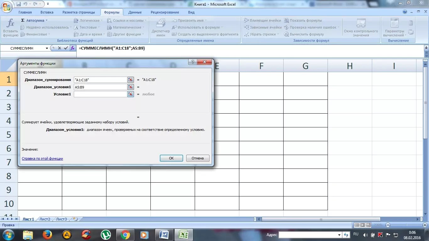
VLOOKUP function

Using the VLOOKUP function, you can extract the necessary information from the tables. The essence of vertical lookup is to look for the value in the leftmost column of the given range.

After that, the total value is returned from the cell, which is located at the intersection of the selected row and column.

The calculation of the VLOOKUP can be seen in an example that shows a list of surnames. The task is to find the last name by the given number.

Applying the VLOOKUP function

The formula shows that the first argument of the function is cell C1.

The second argument A1:B10 is the range to search.

The third argument is the index number of the column from which to return the result.

Calculating a given last name using the VLOOKUP function

In addition, you can search for the last name even if some sequence numbers are missing.

If you try to find the last name from a non-existent number, the formula will not give an error, but will give the correct result.

Search for a last name with missing numbers

This phenomenon is explained by the fact that the VLOOKUP function has a fourth argument, with which you can set the interval view.

It has only two values ​​- "false" or "true". If no argument is given, it defaults to true.

Rounding Numbers with Functions

The functions of the program allow you to accurately round any fractional number up or down.

And the resulting value can be used in calculations in other formulas.

The number is rounded using the ROUNDUP formula. To do this, you need to fill in the cell.

The first argument is 76.375 and the second is 0.

Rounding a number with a formula

In this case, the number has been rounded up. To round a value down, select the ROUNDDOWN function.

Rounding occurs to an integer. In our case, up to 77 or 76.

Excel helps to simplify any calculations. With the help of a spreadsheet, you can complete tasks in higher mathematics.

The program is most actively used by designers, entrepreneurs, as well as students.

The whole truth about Microsoft Excel 2007 formulas

EXCEL formulas with examples - Instructions for use

A formula is a mathematical expression that is created to calculate a result and that may depend on the contents of other cells. A formula in a cell can contain data, references to other cells, and an indication of the action to be taken.

Using cell references allows formula results to be recalculated when the contents of cells included in formulas change.

In Excel, formulas start with an = sign. Parentheses () can be used to specify the order of mathematical operations.

Excel supports the following operators:

• Arithmetic operations:
  • addition (+);
  • multiplication (*);
  • finding the percentage (%);
  • subtraction (-);
  • division (/);
  • exponent (^).
• Comparison operators:
  • = equal;
  • < меньше;
  • > more;
  • <= меньше или равно;
  • >= greater than or equal;
  • <>not equal.
• Telecom operators:
  • : range;
  • ; an association;
  • & text join operator.

Table 22. Formula examples

The exercise

Insert formula -25-A1+AZ

Pre-enter any numbers in cells A1 and A3.

1. Select the desired cell, for example B1.
2. Start entering a formula with the = sign.
3. Enter the number 25 followed by the operator (sign -).
4. Enter a reference to the first operand, for example by clicking on the desired cell A1.
5. Enter the following operator (+ sign).
6. Click in the cell that is the second operand in the formula.
7. Finish entering the formula by pressing the key Enter. In cell B1, get the result.

Autosummation

Button Autosum (AutoSum)- ∑ can be used to automatically create a formula that sums the area of ​​neighboring cells that are directly left in this line and directly above in this column.

1. Select the cell where you want to place the result of the summation.
2. Click the AutoSum - ∑ button or press the keyboard shortcut Alt+=. Excel will decide which area to include in the summation range and highlight it with a dotted moving box called a border.
3. Click Enter to accept the area that Excel has selected, or use the mouse to select a new area and then press Enter.

The AutoSum function automatically transforms when cells are added and removed within the area.

The exercise

Creating a table and calculating by formulas

1. Enter numeric data in the cells, as shown in the table. 23.

	A	V	WITH	D	B	F
1
2		Magnolia	Lily	Violet	Total
3	Higher	25	20	9
4	Average spec.	28	23	21
5	vocational school	27	58	20
v	Other	8	10	9
7	Total
8	Without higher

Table 23. Initial data table

1. Select cell B7, in which the vertical sum will be calculated.
2. Click the AutoSum - ∑ button or click Alt+=.
3. Repeat steps 2 and 3 for cells C7 and D7.

Calculate the number of employees without higher education (using the B7-B3 formula).

1. Select cell B8 and type the (=) sign.
2. Click in cell B7, which is the first operand in the formula.
3. Enter the (-) sign on the keyboard and click in the OT cell, which is the second operand in the formula (the formula will be entered).
4. Click Enter(in cell B8 the result will be calculated).
5. Repeat steps 5-8 to calculate the corresponding formulas in cells C8 and 08.
6. Save the file with the name Education_Employees.x1s.

Table 24Calculation result

	A	B	WITH	D	E	F
1	Distribution of employees by education
2		Magnolia	Lily	Violet	Total
3	Higher	25	20	9
4	Average spec.	28	23	21
5	vocational school	27	58	20
6	Other	8	10	9
7	Total	88	111	59
8	Without higher	63	91	50

Duplicate formulas using the fill handle

A cell area (cell) can be replicated by using fill marker. As shown in the previous section, the fill handle is the breakpoint in the lower right corner of the selected cell.

Often it is necessary to multiply not only data, but also formulas containing address links. The process of replicating formulas using a fill handle allows you to colorize a formula while changing the address references in the formula.

1. Select the cell containing the formula to replicate.
2. Drag fill marker in the right direction. The formula will be duplicated in all cells.

Typically, this process is used when copying formulas within rows or columns containing data of the same type. When replicating formulas using a fill marker, the so-called relative addresses of cells in the formula change (relative and absolute references will be described in detail later).

The exercise

Replication of formulas

1.Open the file Education_Employees.x1s.

1. Enter in cell E3 the formula for autosumming cells = SUM (OT: 03).
2. Drag and drop the fill handle to copy the formula into cells E4:E8.
3. See how the relative cell addresses change in the resulting formulas (Table 25) and save the file.

	A	V	WITH	D	E	F
1	Distribution of employees by education
2		Magnolia	Lily	Violet	Total
3	Higher	25	20	9	=SUM(VZ:03)
4	Average spec.	28	23	21	=SUM(B4:04)
5	vocational school	27	58	20	=SUM(B5:05)
6	Other	8	10	9	=SUM(B6:06)
7	Total	88	111	58	=SUM(B7:07)
8	Without higher	63	91	49	=SUM(B8:08)

Table 25. Changing cell addresses when replicating formulas

Relative and absolute links

Formulas that implement calculations in tables use so-called links to address cells. Cell reference can be relative or absolute.

The use of relative references is similar to indicating the direction of travel along the street - "go three blocks north, then two blocks west." Following these instructions from different starting places will lead to different destinations.

For example, a formula that sums the numbers in a column or row is then often copied to other row or column numbers. These formulas use relative references (see the previous example in Table 25).

An absolute cell reference. Go cell area will always refer to the same row and column address. When compared with the directions of the streets, it will be something like this: "Go to the intersection of the Arbat and the Boulevard Ring." Regardless of the starting point, this will lead to the same place. If the formula requires that the cell address remain unchanged when copied, then an absolute reference (record format $A$1) must be used. For example, when a formula calculates fractions of a total, the reference to the cell containing the total must not change when copied.

A dollar sign ($) will appear before both a column reference and a row reference (e.g. $C$2), Successive pressing F4 will add or remove a sign before the column or row number in the reference (C$2 or $C2 - the so-called mixed links).

1. Create a table similar to the one below.

Table 26. Payroll

1. In the SZ cell, enter the formula for calculating Ivanov's salary \u003d V1 * VZ.

When replicating the formula of this example with relative references in cell C4, an error message (#VALUE!) appears, since the relative address of cell B1 will change, and the formula =B2*B4 will be copied to cell C4;

1. Set the absolute reference to cell B1 by placing the cursor in the formula bar on B1 and pressing the F4 key. The formula in cell C3 will look like =$B$1*B3.
2. Copy the formula into cells C4 and C5.
3. Save the file (Table 27) under the name Salary.xls.

Table 27. Payroll results

Names in formulas

Names in formulas are easier to remember than cell addresses, so you can use named scopes (single or multiple cells) instead of absolute references. The following rules must be observed when creating names:

• names can be up to 255 characters long;
• names must begin with a letter and may contain any character except a space;
• names should not look like links, such as OT, C4;
• names should not use Excel functions such as SUM IF etc.

On the menu Insert, Name There are two different commands for creating named areas: Create and Assign.

Team Create allows you to set (enter) the required name ( only one), Assign command uses the labels placed on the worksheet as area names (it is allowed to create several names at once).

Making a name

1. Select cell B1 (Table 26).
2. Select from the menu Insert, Name (Insert, Name) command Assign (Define).
3. Enter your name Hourly rate and click OK.
4. Select cell B1 and make sure the name field says hourly rate.

Creating multiple names

1. Select cells ВЗ:С5 (Table 27).
2. Select from the menu Insert, Name (Insert, Name) command Create (Create), a dialog box will appear. Create names(Fig. 88).
3. Make sure the radio button in the column on the left is checked and click OK.
4. Highlight the cells OT:NW and make sure the name field says Ivanov.

Rice. Figure 88. Create Names Dialog Box

You can insert a name into a formula instead of an absolute reference.

1. In the formula bar, position the cursor where the name will be added.
2. Select from the menu Insert, Name (Insert, Name) command Paste (Paste), The Insert Names dialog box appears.

1. Select the desired name from the list and click OK.

Errors in formulas

If an error is made when entering formulas or data, an error message appears in the resulting cell. The first character of all error values ​​is #. Error values ​​depend on the type of error made.

Excel can recognize far from all errors, but those that are found must be able to correct.

Error # # # # appears when the entered number does not fit in the cell. In this case, increase the column width.

Error #DIV/0! appears when an attempt is made to divide by zero in a formula. This most often happens when the divisor is a cell reference that contains a zero or blank value.

Error #N/A! is an abbreviation for "undefined data". This error indicates the use of an empty cell reference in the formula.

Error #NAME? appears when a name used in a formula has been removed or was not previously defined. To correct, define or correct the data area name, function name, etc.

Error #BLANK! appears when the intersection of two regions is specified, which do not actually have common cells. Most often, the error indicates that an error was made when entering cell range references.

Error #NUMBER! appears when an invalid format or argument value is used in a function with a numeric argument.

Error #VALUE! appears when an invalid argument or operand type is used in a formula. For example, text is entered instead of a numeric or boolean value for an operator or function.

In addition to the errors listed above, when entering formulas, a circular reference may appear.

A circular reference occurs when a formula directly or indirectly includes references to its own cell. A circular reference can cause distortion in worksheet calculations and is therefore considered a bug in most applications. When entering a circular reference, a warning message appears (Fig. 89).

To correct the error, delete the cell that caused the circular reference, edit or re-enter the formula.

Functions in Excel

More complex calculations in Excel tables are carried out using special functions (Fig. 90). The list of function categories is available when you select the command Function in the Insert menu (Insert, Function).

Financial functions perform such calculations as calculating the amount of payment on a loan, the amount of payment of profit on investments, etc.

The Date and Time functions allow you to work with date and time values ​​in formulas. For example, you can use the current date in a formula by using the function TODAY.

Rice. 90. Function Wizard

Math functions perform simple and complex mathematical calculations, such as calculating the sum of a range of cells, the absolute value of a number, rounding numbers, etc.

Statistical functions allow you to perform statistical analysis of the data. For example, you can determine the mean and variance of a sample, and much more.

Database Functions can be used to perform calculations and to select records by condition.

Text functions provide the user with the ability to process text. For example, you can concatenate multiple strings using the function CONNECT.

Boolean functions are designed to test one or more conditions. For example, the IF function allows you to determine whether the specified condition is true, and returns one value if the condition is true, and another value if it is false.

Functions Checking properties and values are intended to define the data stored in the cell. These functions check the values ​​in the cell according to the condition and return the values ​​depending on the result. TRUE or FALSE.

For table calculations using built-in functions, we recommend using the Function Wizard. The function wizard dialog box is available when you select the command Function in the Insert menu or pressing a button , on the standard toolbar. During the dialogue with the wizard, it is required to set the arguments of the selected function; for this, it is necessary to fill in the fields in the dialog box with the corresponding values ​​or addresses of the table cells.

The exercise

Calculation of the average value for each line in the file Education.xls.

1. Highlight cell F3 and click on the Function Wizard button.
2. In the first dialog box of the Function Wizard, from the Statistical category, select a function AVERAGE, click on the button Further.
3. Arguments must be given in the second dialog box of the function wizard. The input cursor is in the input field of the first argument. In this field as an argument number! enter the address of the range B3:D3 (Fig. 91).
4. Click OK.
5. Copy the resulting formula into cells F4:F6 and save the file (Table 28).

Rice. 91 Entering an Argument in the Function Wizard

Table 28. Table of calculation results using the function wizard

	A	V	WITH	D	E	F
1	Distribution of employees by education
2		Magnolia	Lily	Violet	Total	The average
3	Higher	25	20	9	54	18
4	Average spec.	28	23	21	72	24
8	vocational school	27	58	20	105	35
v	Other	8	10	9	27	9
7	Total	88	111	59	258	129

To enter a range of cells in the function wizard window, you can circle this range on the worksheet of the table (in the example B3:D3). If the Function Wizard window covers the desired cells, you can move the dialog box. After selecting a range of cells (B3:D3), a running dotted frame will appear around it, and the address of the selected range of cells will automatically appear in the argument field.

Formulas in Excel are one of the most important advantages of this editor. Thanks to them, your possibilities when working with tables increase several times and are limited only by the available knowledge. You can do anything. At the same time, Excel will help at every step - in almost any window there are special tips.

To create a simple formula, just follow the following instructions:

1. Make any cell active. Click on the formula entry bar. Put an equal sign.

1. Enter any expression. Can be used as numbers

In this case, the affected cells are always highlighted. This is done so that you do not make a mistake with the choice. It is easier to see the error visually than in text form.

What is the formula

Let's take the following expression as an example.

It consists of:

• the symbol "=" - any formula begins with it;
• "SUM" function;
• function argument "A1:C1" (in this case, it is an array of cells from "A1" to "C1");
• operator "+" (addition);
• links to cell "C1";
• operator "^" (exponentiation);
• constants "2".

Using Operators

Operators in the Excel editor indicate exactly what operations to perform on the specified elements of the formula. The calculation always follows the same order:

• parentheses;
• exhibitors;
• multiplication and division (depending on the sequence);
• addition and subtraction (also depending on the sequence).

Arithmetic

These include:

• addition - "+" (plus);

=2+2

• negation or subtraction - "-" (minus);

=2-2 =-2

If you put a minus in front of the number, then it will take a negative value, but the absolute value will remain exactly the same.

• multiplication - "*";

=2*2

• division "/";

=2/2

• percent "%";

=20%

• exponentiation - "^".

=2^2

Comparison Operators

These operators are used to compare values. The operation returns TRUE or FALSE. These include:

• the sign of "equality" - "=";

=C1=D1

• greater than sign - ">";

=C1>D1

• less sign -<»;

=C1

the sign "greater than or equal to" - ">=";

=C1>=D1

• less than or equal sign<=»;

=C1<=D1

• "not equal" sign<>».

=C1<>D1

Text concatenation operator

The special character "&" (ampersand) is used for this purpose. With it, you can connect different fragments into one whole - the same principle as with the "CONNECT" function. Here are some examples:

1. If you want to combine text in cells, then you need to use the following code.

=A1&A2&A3

1. In order to insert some character or letter between them, you need to use the following construction.

=A1&","&A2&","&A3

1. You can combine not only cells, but also ordinary characters.

="Auto"&"Mobile"

Any text other than links must be enclosed in quotation marks. Otherwise, the formula will throw an error.

Please note that quotes are used exactly as in the screenshot.

You can use the following operators to define links:

• in order to create a simple link to the desired range of cells, it is enough to specify the first and last cell of this area, and the “:” symbol between them;
• to combine links, use the sign ";";
• if it is necessary to determine the cells that are at the intersection of several ranges, then a “space” is placed between the links. In this case, the value of the cell "C7" will be displayed.

Since only it falls under the definition of "intersection of sets." This is the name of this operator (space).

Use of links

While working in the Excel editor, you can use links of various kinds. However, most novice users know how to use only the simplest of them. We will teach you how to correctly enter links of all formats.

Simple Links A1

As a rule, this type is used most often, since it is much more convenient to compose them than the rest.

• columns - from A to XFD (no more than 16384);
• lines - from 1 to 1048576.

Here are some examples:

• cell at the intersection of row 5 and column B - "B5";
• range of cells in column B starting from row 5 to row 25 - "B5:B25";
• the range of cells in row 5 starting from column B to F - "B5:F5";
• all cells in row 10 - "10:10";
• all cells in rows 10 to 15 - "10:15";
• all cells in column B - "B:B";
• all cells in columns from B to K - "B:K";
• the range of cells from B2 to F5 is "B2-F5".

Sometimes formulas use information from other sheets. It works as follows.

=SUM(Sheet2!A5:C5)

The second sheet contains the following data.

If there is a space in the sheet name, then in the formula it must be indicated in single quotes (apostrophes).

=SUM("Sheet number 2"!A5:C5)

Absolute and relative links

The Excel editor works with three types of links:

• absolute;
• relative;
• mixed.

Let's consider them more carefully.

All of the previously mentioned examples belong to relative cell addresses. This type is the most popular. The main practical advantage is that the editor will change the references to a different value during the migration. In accordance with where exactly you copied this formula. For the calculation, the number of cells between the old and new position will be taken into account.

Imagine that you need to stretch this formula to the entire column or row. You will not manually change letters and numbers in cell addresses. It works as follows.

1. Enter the formula for calculating the sum of the first column.

=SUM(B4:B9)

1. Press the hotkeys Ctrl +C . In order to transfer the formula to the next cell, you need to go there and press Ctrl + V .

If the table is very large, it is better to click on the lower right corner and, without releasing your finger, stretch the pointer to the end. If there is little data, then copying using hotkeys is much faster.

1. Now look at the new formulas. The change in the column index happened automatically.

If you want all links to be preserved when transferring formulas (that is, so that they do not change automatically), you need to use absolute addresses. They are specified as "$B$2".

=SUM($B$4:$B$9)

As a result, we see that no changes have occurred. All columns display the same number.

This type of address is used when it is necessary to fix only a column or row, and not all at the same time. You can use the following constructs:

• $D1, $F5, $G3 - for fixing columns;
• D$1, F$5, G$3 - to fix rows.

Work with such formulas only when necessary. For example, if you need to work with one constant row of data, but only change the columns. And most importantly - if you are going to calculate the result in different cells that are not located along the same line.

The fact is that when you copy the formula to another line, the numbers in the links will automatically change by the number of cells from the original value. If you use mixed addresses, then everything will remain in place. This is done in the following way.

1. Let's use the following expression as an example.

=B$4

1. Let's move this formula to another cell. Preferably not on the next and on another line. Now you can see that the new expression contains the same string (4) but a different letter, since it was the only one that was relative.

3D Links

The concept of "three-dimensional" includes those addresses in which a range of sheets is indicated. An example formula looks like this.

=SUM(Sheet1:Sheet4!A5)

In this case, the result will correspond to the sum of all cells "A5" on all sheets, starting from 1 to 4. When compiling such expressions, the following conditions must be observed:

• arrays cannot use such references;
• three-dimensional expressions are forbidden to be used where there is an intersection of cells (for example, the "space" operator);
• when creating formulas with 3D addresses, you can use the following functions: AVERAGE, STDEV, STDEV.V, AVERAGE, STDEV, STDEV.Y, SUM, COUNT, COUNT, MIN, MAX, MIN, MAX, VARR, PRODUCT, VARV, VAR.V and DISPA.

If you violate these rules, then you will see some kind of error.

R1C1 format links

This type of links differs from "A1" in that the number is given not only to rows, but also to columns. The developers decided to replace the normal view with this option for convenience in macros, but they can be used anywhere. Here are some examples of such addresses:

• R10C10 is an absolute link to the cell, which is located on the tenth line of the tenth column;
• R - absolute link to the current (in which the formula is indicated) link;
• R[-2] – relative link to the line, which is located two positions above this one;
• R[-3]C – relative reference to the cell, which is located three positions higher in the current column (where you decided to write the formula);
• RC is a relative link to the cell that is five cells to the right and five lines below the current one.

Name usage

The Excel program for naming cell ranges, single cells, tables (regular and summary), constants and expressions allows you to create your own unique names. At the same time, there is no difference for the editor when working with formulas - he understands everything.

You can use the names for multiplication, division, addition, subtraction, calculation of interest, ratios, deviations, rounding, VAT, mortgages, loans, estimates, timesheets, various forms, discounts, salaries, seniority, annuity payments, working with VLOOKUP formulas , "VVD", "INTERIM. RESULTS" and so on. That is, you can do whatever you want.

Only one thing can be called the main condition - you must determine this name in advance. Otherwise, Excel will not know anything about it. This is done in the following way.

1. Select a column.
2. Call the context menu.
3. Select "Give Name".

1. Specify the desired name for this object. In this case, you must adhere to the following rules.

1. Click the "OK" button to save.

In the same way, you can assign a name to any cell, text or number.

You can use the information in the table both with the help of names and with the help of ordinary links. This is what the standard looks like.

And if you try to insert our name instead of the address "D4: D9", you will see a hint. It is enough to write a few characters, and you will see what fits (from the name base) the most.

In our case, everything is simple - “column_3”. And imagine that you will have a large number of such names. You won't be able to memorize everything.

Using functions

There are several ways to insert a function in the Excel editor:

• manually;
• using the toolbar;
• using the Insert Function window.

Let's take a closer look at each method.

In this case, everything is simple - you use your hands, your own knowledge and skills to enter formulas in a special line or directly in a cell.

If you do not have working experience in this area, then it is better to use more lightweight methods at first.

In this case it is necessary:

1. Go to the "Formulas" tab.
2. Click on any library.
3. Select the desired function.

1. Immediately after that, the "Arguments and Functions" window will appear with the function already selected. You just have to put down the arguments and save the formula using the "OK" button.

Substitution Wizard

You can apply it like this:

1. Make any cell active.
2. Click on the "Fx" icon or use the keyboard shortcut SHIFT + F3.

1. Immediately after that, the "Insert Function" window will open.
2. Here you will see a large list of different features sorted by category. In addition, you can use the search if you can not find the desired item.

It is enough to score a word that can describe what you want to do, and the editor will try to display all the appropriate options.

1. Select any function from the proposed list.
2. To continue, you need to click on the "OK" button.

1. You will then be asked for "Arguments and Functions". You can do this manually or simply select the desired range of cells.
2. In order to apply all the settings, you need to click on the "OK" button.

1. As a result of this, we will see the number 6, although this was already understandable, since the Arguments and Functions window displays a preliminary result. The data is recalculated instantly when any of the arguments changes.

Using nested functions

As an example, we will use formulas with logical conditions. To do this, we will need to add some kind of table.

Then follow the instructions below:

1. Click on the first cell. Call the "Insert function" window. Select the "If" function. Click "OK" to paste.

1. Then you will need to compose some kind of logical expression. It must be written in the first field. For example, you can add the values ​​of three cells in one row and check if the sum is greater than 10. In the case of "true", specify the text "More than 10". For a false result - "Less than 10". Then click OK to return to the workspace.

1. As a result, we see the following - the editor gave out that the sum of the cells in the third row is less than 10. And this is correct. So our code is working.

=IF(SUM(B3:D3)>10,"Greater than 10","Less than 10")

1. Now you need to configure the following cells. In this case, our formula simply extends further. To do this, you first need to move the cursor to the lower right corner of the cell. After the cursor changes, you need to make a left click and copy it to the very bottom.

1. As a result, the editor recalculates our expression for each line.

As you can see, the copy was very successful because we used the relative links we talked about earlier. If you need to fix addresses in function arguments, then use absolute values.

There are several ways to do this: use the formula bar or a special wizard. In the first case, everything is simple - click in a special field and manually enter the necessary changes. But writing there is not very convenient.

The only thing you can do is increase the input field. To do this, just click on the indicated icon or press the key combination Ctrl + Shift + U.

It is worth noting that this is the only way if you do not use functions in the formula.

In the case of using functions, everything becomes much simpler. To edit, follow the instructions below:

1. Make active the cell with the formula. Click on the "Fx" icon.

1. After that, a window will appear in which you can change the arguments of the function you need in a very convenient way. In addition, here you can find out exactly what the result of recalculating the new expression will be.

1. To save the changes made, use the "OK" button.

To remove an expression, just do the following:

1. Click on any cell.

1. Click on the Delete or Backspace button. As a result, the cell will be empty.

You can achieve exactly the same result using the Clear All tool.

Possible errors when compiling formulas in the Excel editor

The following are the most common mistakes that users make:

• The expression uses a huge number of nestings. There should be no more than 64;
• paths to external workbooks are specified in formulas without the full path;
• Opening and closing parentheses are misplaced. That is why in the editor in the formula bar all brackets are highlighted in a different color;

• the names of books and sheets are not taken in quotation marks;
• numbers are used in the wrong format. For example, if you need to specify $2000, you just need to type 2000 and select the appropriate cell format, since the $ symbol is used by the program for absolute references;

• required function arguments are not specified. Note that optional arguments are enclosed in square brackets. Everything without them is necessary for the full operation of the formula;

• Cell ranges are incorrect. To do this, you must use the ":" (colon) operator.

Error codes when working with formulas

When working with a formula, you may see the following error options:

• #VALUE! - This error indicates that you are using the wrong data type. For example, you are trying to use text instead of a numeric value. Of course, Excel can't calculate the sum between two phrases;
• #NAME? - a similar error means that you made a typo in the spelling of the function name. Or you are trying to enter something that does not exist. You can't do that. In addition, the problem may be in another. If you are sure about the function name, then try to look at the formula more closely. Perhaps you forgot a parenthesis. In addition, you need to take into account that text fragments are indicated in quotation marks. If all else fails, try composing the expression again;
• #NUMBER! - displaying such a message means that you have some kind of problem with the arguments or with the result of the formula. For example, the number turned out to be too large or vice versa - small;
• #DIV/0! - This error means that you are trying to write an expression that divides by zero. Excel cannot undo math rules. Therefore, such actions are also prohibited here;
• #N/A! - The editor can show this message if some value is not available. For example, if you use the functions SEARCH, SEARCH, MATCH, and Excel did not find the fragment you are looking for. Or there is no data at all and the formula has nothing to work with;
• If you are trying to calculate something and Excel writes the word #REF!, then the wrong range of cells is used in the function argument;
• #EMPTY! - this error appears if you have an inconsistent formula with overlapping ranges. More precisely, if in reality there are no such cells (which are at the intersection of two ranges). Quite often, this error occurs by accident. It is enough to leave one space in the argument, and the editor will perceive it as a special operator (we talked about it earlier).

When editing the formula (the cells are highlighted) you will see that they do not actually intersect.

Sometimes you can see a lot of # characters that completely fill the width of the cell. In fact, there is no error here. This means that you are working with numbers that do not fit in this cell.

In order to see the value contained there, it is enough to resize the column.

In addition, you can use cell formatting. To do this, you need to follow a few simple steps:

1. Call the context menu. Select Format Cells.

1. Specify the type "General". Use the "OK" button to continue.

Thanks to this, the Excel editor will be able to translate this number into another format that fits in this column.

Formula Usage Examples

The Microsoft Excel editor allows you to process information in any way convenient for you. There are all necessary conditions and opportunities for this. Let's look at some examples of formulas by categories. This will make it easier for you to figure it out.

In order to evaluate the mathematical capabilities of Excel, you need to perform the following steps.

1. Create a table with some conditional data.

1. To calculate the amount, enter the following formula. If you only want to add one value, you can use the addition ("+") operator.

=SUM(B3:C3)

1. Oddly enough, in the Excel editor you can not take away using functions. For deduction, the usual operator "-" is used. In this case, the code will be the following.

=B3-C3

1. In order to determine how much the first number is from the second as a percentage, you need to use this simple construction. If you want to subtract several values, you will have to write a "minus" for each cell.

=B3/C3%

Note that the percent symbol is placed at the end, not at the beginning. In addition, when working with percentages, you do not need to additionally multiply by 100. This happens automatically.

1. Excel can add, taking into account several conditions at once. You can calculate the sum of the cells of the first column, the value of which is greater than 2 and less than 6. And the same formula can be set for the second column.

=SUMIFS(B3:B9,B3:B9,">2",B3:B9,"<6") =SUMIFS(C3:C9,C3:C9,">2",C3:C9,"<6")

1. You can also count the number of elements that satisfy some condition. For example, let Excel calculate how many numbers we have greater than 3.

=COUNTIF(B3:B9,">3") =COUNTIF(C3:C9,">3")

1. The result of all formulas will be as follows.

Math functions and graphs

Using Excel, you can calculate various functions and build graphs on them, and then carry out graphical analysis. As a rule, such techniques are used in presentations.

As an example, let's try to build graphs for the exponent and some equation. The instruction will be as follows:

1. Let's create a table. In the first column we will have the original number "X", in the second - the "EXP" function, in the third - the specified ratio. It would be possible to make a quadratic expression, but then the resulting value against the background of the exponent on the graph would practically disappear.

As we said earlier, the growth of the exponent is much faster than that of the usual cubic equation.

Similarly, any function or mathematical expression can be represented graphically.

Everything described above is suitable for modern programs of 2007, 2010, 2013 and 2016. The old Excel editor is significantly inferior in terms of features, number of functions and tools. If you open the official help from Microsoft, you will see that they additionally indicate in which version of the program this function appeared.

In all other respects, everything looks almost exactly the same. As an example, let's calculate the sum of several cells. For this you need:

1. Specify some data for calculation. Click on any cell. Click on the "Fx" icon.

1. Select the "Math" category. Find the "SUM" function and click on "OK".
1. You can try to recalculate in any other editor. The process will be exactly the same.

Conclusion

In this tutorial, we talked about everything related to formulas in the Excel editor, from the simplest to the very complex. Each section was accompanied by detailed examples and explanations. This is done so that the information is accessible even for complete dummies.

If something does not work out for you, then you are making a mistake somewhere. Perhaps you have typos in expressions or incorrect cell references. The main thing to understand is that everything needs to be driven in very carefully and carefully. Moreover, all functions are not in English, but in Russian.

In addition, it is important to remember that formulas must begin with the symbol "=" (equal to). Many novice users forget about it.

Sample File

In order to make it easier for you to deal with the formulas described earlier, we have prepared a special demo file in which all the above examples were compiled. You can do it from our site absolutely free. If during training you use a ready-made table with formulas based on the data you filled in, you will achieve results much faster.

Video instruction

If our description did not help you, try watching the attached video below, which tells the main points in more detail. Perhaps you are doing everything right, but you are missing something. With the help of this video, you should deal with all the problems. We hope these tutorials have helped you. Check us out more often.

The main purpose of Excel is to perform calculations on data. Data processing occurs in cells containing formulas. You have already studied the rules for entering the simplest formulas at the beginning of the section. In this subsection, we will consider the general principles for creating formulas of any complexity and study examples of typical calculations in Excel.

Rules for entering formulas

Any formula must always be entered with an equals sign "=". The formula may contain:

signs of arithmetic operations: "+", "-", "*", "/", "^" (sign of raising a number to a power), sign "%";

numbers, strings (they are taken in quotes);

references to cells and ranges of cells (both on the current sheet and on other sheets of the book) to determine the order of calculations, brackets;

built-in functions.

Excel has a large number of functions with which you can perform calculations and other actions related to a wide variety of areas of knowledge. When using a built-in function, after the "=" sign, you should enter its name, and then in brackets the arguments of the function - the data that are used in the calculations. Function arguments can be numbers, cell references or cell ranges, or other built-in functions (called nested functions). Consider specific examples:

А2+В2 - addition of values ​​of two cells;

A1 * 0.8 - multiplying the number from cell A1 by 0.8;

D1^2+1 - squaring the number from cell D1 and adding one to the result;

SUM(A1:A5) - summing values ​​from the range of cells A1:A5. This is an example of using a built-in function. Here SUM is the name of the function, A1:A5 is the range of cells, its only argument enclosed in brackets;

MULTIP(B1:B2;B7:C7) - calculation of the product of matrices B1:B2 and B7:C7. As you can see, this function has two arguments, which are arrays of data from the selected ranges. If a function has multiple arguments, they are separated from each other by a semicolon. You can use cell and range references on the current sheet and other sheets as function arguments. In the latter case, before the address of the cell or range, enter the name of the sheet, separated by dashes, and put the separator "!", For example, 'Sheet1'!B2, 'Sheet 3'!A1:C4. A stroke can be entered by pressing the "E" key with the active English layout.

Of course, it is impossible to remember the syntax of all the built-in functions in Excel, and you don't need to do this, because in everyday practice you will use only a few built-in functions to solve the most common tasks.

The options for inserting inline functions into a document are located on the Formulas tab in the Function Library group. Functions are divided into categories depending on what types of tasks they are intended for. The purpose of a particular function can be read on the tooltip that appears when you hover the mouse pointer over the name of a function with a menu (Fig. 17).

If you want to see the full list of Excel's built-in functions, click the Insert Function button found in the formula bar. In the Function Wizard window that opens, select Full alphabetical listing from the Category drop-down list and click on the name of the function to read below about the actions it performs.

The name of a built-in function can be entered from the keyboard (which is highly undesirable due to the high probability of error), inserted from the corresponding menu of buttons located in the Function Library group on the Formulas tab, or from the Function Wizard window. The last two options will be discussed below.

Rice. 17. View function assignment

The functions that are often used in practice are placed in the button menu, which is located in the Editing group on the Home tab. Consider the tasks associated with their use.

The simplest calculations

The function of summarizing data is the most popular, which is why it is the easiest to use it in Excel.

If the data is in one column or row, select it and click the button. The result of the addition is immediately displayed at the bottom (in the case of a column) or to the right (in the case of a row) of the row. Click on it, and in the formula bar you will see that Excel has used the =SUM() function.

If you need to sum the values ​​from several rows or columns (whether they are adjacent or not), select the rows and use this button again. The amounts will immediately be displayed in the next cell next to it.

To sum cells that are in a rectangular area or in different parts of a document, do the following:

1. Click on the cell where you want to display the result of the summation.

2. Press the button. This will place the summation function in the cell, and the cursor in its parentheses will blink, indicating that you need to enter arguments.

3. Select the desired range of cells (if necessary - several ranges by holding down the key). In this case, it will be covered by a running frame, and links to cell ranges will appear in the formula brackets (Fig. 18).

4. Click to get the result.

Rice. 18. Sum a range of cells

Even after the formula has been entered, you can always edit it by changing or adding arguments or functions. So, to change the range of cells in the example just discussed, proceed as follows.

1. Double click on the cell containing the formula. In this case, the range taking part in the calculations will be covered by a blue frame with markers in the corners.

2. Move the mouse pointer to the desired corner and, when it becomes a double-headed arrow, drag the borders of the frame so as to capture new cells (or, conversely, exclude old ones). In this case, the address of the range in brackets of the formula will change automatically.

3. Click to calculate a new result.

Clicking on the button's arrow will reveal a list of commands that call functions that can be used as quickly as the summation function. The scheme of actions when using them does not differ from the sequence of steps for the summation function. The following is a brief description of the functions called by the button commands.

The average. Calls the function =AVERAGE(), which can be used to calculate the arithmetic average of a range of cells (to sum all the data, and then divide by their number).

Number. Calls the function =COUNT(), which determines the number of cells in the selected range.

Maximum. Calls the =MAX() function, which can be used to determine the largest number in the selected range.

Minimum. Calls the =MIN() function to find the smallest value in the selected range.

The result of the work of some of the listed functions can be seen without referring directly to the functions themselves. Highlight the range you are interested in and look down at the Excel status bar. To the left of the scale control, the values ​​of the sum, the number of cells in the range, and the arithmetic mean will appear (Fig. 19).

Complex calculations

You have studied examples of the simplest calculations in Excel. Now try to deal with a complex task that requires a combination of the actions we considered earlier.

Task 1. Select the optimal tariff plan when connecting to a cellular network, if 2.5 hours of calls within the network and 0.5 hours of calls with subscribers of the city network and other cellular operators are planned per month. Prices for services are presented in the table in fig. 20 excluding VAT.

First of all, you need to create a table and enter prices for the services of cellular operators into it, as it is done in Fig. 20. To calculate the final amount including VAT, a separate column should be marked at the end of the table.

Select cell A1 and type the name of the work in it. In the cells of the next row, create table headers. Use the Wrap Text button in the Alignment group to adjust the line height. Adjust the width of the columns manually by dragging the borders of their headers. Using the alignment buttons, place the text in the "header" in the middle (relative to the top and bottom borders of the cell) and in the center (relative to the left and right borders).

Next, fill in the table grid with the values ​​shown in Fig. 20. Since the tariffs are presented per minute of communication, the planned talk time must also be entered in minutes in the columns Calls within the network and Calls to other networks. You do not need to fill in both columns manually. It is enough to enter the value in the first cell, and then copy it to the rest using autocomplete.

In the last column Total, including VAT 18%, there will be calculation formulas, which we will now begin to create. At the bottom of the column, create a heading called Optimum, below which you place a function to calculate the minimum value of the series to determine the lowest cost. To do this, click on the button arrow, activate the Minimum command, select the range of still empty cells in the Total column including 18% VAT and click.

The total costs will consist of the subscription fee, the cost of calls within the network and with subscribers of other networks, as well as value added tax. This needs to be presented as a formula. Let's start the calculations with the first tariff plan Minutka. To the contents of cell B3 (monthly fee), you need to add the product of cells C3 and E3 (total cost of calls within the network) and the product of cells D3 and F3 (total cost of calls to subscribers of other networks). This will calculate the total cost excluding VAT. To add the tax rate to the amount received, you need to multiply the result by 18% and add it to the cost of services. This is the result and should appear in the cells of the last column.

Select cell G3, type the "=" sign in it and press the button. In this case, the summation function will be inserted, the range of cells will be automatically determined, and its address will be highlighted in the brackets of the function. Since this range does not suit us, click to remove the link from the brackets. Then click on cell B3 to put its address in the formula and put ";" to separate the next argument (term). Next, click on cell C3 to enter a reference to it in the formula, type the multiplication sign "*" and select cell E3. Separate the new argument with a semicolon. To enter the last term, click on cell D3, enter "*" and select cell F3. So we created a part of the formula that is responsible for calculating the total costs excluding taxes. It should look like this: =SUM(B3;C3*E3;D3*F3). If you make a mistake somewhere, position the cursor next to it with a mouse click or using the movement keys and make corrections. Next, you need to add the tax part of the formula. Move the cursor to the end of the bracket and type "+". The VAT rate is 18%. Therefore, you need to multiply 18% by the result obtained in the first part of the formula. Type 18% and the multiplication sign "*", then select the first part of the formula, not including the "=" sign (just like you would select a text fragment in Word), right-click on it and use the Copy command of the context menu. Click to position the cursor at the end of the formula, right-click and access the Paste command. The calculation formula is ready: =SUM(B3;C3*E3;D3*F3)+18%*SUM(B3;C3*E3;D3*F3). Click to see the total.

You do not need to manually type the formula in the remaining cells. Use autocomplete - select the cell with the formula and drag the frame down by the marker. As a result, the formula will be copied to the lower cells, and the links in it will automatically be replaced with cell addresses from the same row.

Please note that the minimum amount of expenses was automatically calculated. In our case, it corresponds to the tariff plan Be in touch. Try to change the initial conditions of the task and set a different number of planned minutes of calls within the network and with subscribers of other operators. The recalculation of the total costs will be performed instantly, and it is likely that a different tariff plan will be optimal for the new values.

At the end of the work, format the table so that it looks presentable. First of all, it is worth converting the cells with tariffs to the monetary format. To do this, select all ranges with monetary values ​​in the Monthly fee, Minute within the network, Minute to other networks, Total including 18% VAT and Optimum columns, click on the arrow of the Numeric format drop-down list in the Number group and select the Monetary item. The selected cells will be converted to currency, but since Excel displays two decimal places by default, each number will end with a non-significant zero. To hide it, select the ranges and click the Decrease bit depth button. For some cells, you may also want to hide the second zero after the decimal point. You can do this in a similar way.

Now apply one of the built-in styles to the table. To do this, select the table rectangle itself, not including the name of the task and the optimal calculation cells, click the Format as Table button in the Styles group and select the sketch you like. In the window that appears, select the checkbox Table with headers and click OK. If necessary, reduce the width of the columns by dragging the borders of the headings.

Finally, format the title of the task and the cell with the final result. Select the cells to which the name extends along the length, and click on the button arrow and use the Merge Cells command. Then set specific font options and background color for the cell with the name using the tools of the Font group or apply one of the styles to it using the Cell Styles button in the Styles group. Make out the “header” of the cell with the optimal amount. After performing all the formatting operations, the table with the calculation should take the form similar to that shown in Fig. 21.

Relative and absolute addressing

Cell and range addresses in Excel can be relative or absolute. So far, we've talked about relative cell and range references that only consist of a row number and a column letter, such as B2 or D4:D8. The advantage of relative addressing is that when you copy cells and use autocomplete, the references in the copied formulas change automatically (refer to the cells of the current row, not the original row), so there is no need to manually type each formula. An illustrative example: in the previous example, we typed only one formula in the first cell of the Total column, including 18% VAT, and then used autocomplete. However, in practice, there are situations when the address of a cell or range needs to be fixed so that it does not change when cells are copied or autofilled. To do this, add a "$" sign in front of the row number and column letter. So, if you make the address of cell B2 absolute, it will look like $B$2. It is also possible to fix in the link the address of only the column ($B2) or only the row (B$2). This is called mixed addressing. To quickly change addressing in a ready-made formula, double-click on it, place the cursor on the desired link and press the key in succession to change the address type. The "$" sign can also be added to formulas manually from the keyboard.

Consider the use of absolute addressing on a specific example.

Let's imagine the following situation. You are a wholesale supplier and are ready to provide a discount for some groups of goods that are in stock. The size of the discount varies depending on how well you negotiate with the buyer. After negotiations, you must provide him with a price list, in which the prices will be adjusted for the discount, and further calculations can be made on them.

First of all, you need to create the price list itself with standard prices, in one of the cells type in the percentage of the discount (it can later be varied), and also designate a column in the cells of which there will be formulas that calculate the cost of the goods, taking into account the discount. An example of such a price list is shown in fig. 22. We will omit the description of the design details, since you have already acquired certain skills in this matter. Let's get to the heart of the problem.

To calculate the discounted price, you need to subtract the discount percentage from the current price. In our example, it is equal to ten. At first glance, the solution of the problem is very similar to the previous one, where the VAT percentage was added. Looking at fig. 22, we can assume that in cell C4 it is necessary to subtract the discount from the price in cell B4, which is the product of the size of the discount from cell C1 and the price of the product (B4). In the form of a formula, this will be written as \u003d B4 - C1 * B4. All that remains is to propagate the formula to the remaining cells of the column using autocomplete. Try to follow the described steps, and eventually you will find that there was an error in the calculations. And it consists in the following.

With AutoComplete, cell references automatically change as formulas are copied. In our case, the formula entered in the first cell of the price list was correct, but when we tried to spread it to the other cells of the column, the reference to the cell with the discount size began to change “sliding down” (turning into C2, C3, etc.). To prevent this from happening, its address must be fixed - made absolute. To do this, double-click (C4) on the first cell of the discount column, place the cursor on the address of the cell where the discount value is located (in our case, this is cell C1) and press the key. In this case, the $ ($C$1) sign will be added to the row number and column letter, and the cell address will become absolute - it will not change when the column is autofilled. As a result, the final formula will look like this: \u003d B4 - $ C $ 1 * B4. Now you can repeat the autocomplete procedure to get the correct result. Click on any cell in the discount column to ensure that the absolute reference remains unchanged. When changing the discount value, the entire row will be automatically recalculated.

It is much clearer to use instead of an absolute reference containing the "$" signs, the name of the cell, which can be assigned as follows: select the cell by clicking and type a unique name for it in the formula bar on the left. Click on cell C1 (where the discount amount is indicated), on the left in the formula bar, type Discount. Then, in the first cell of the discounted price column, correct the absolute reference $C$1 to the cell name Discount. The result should be the formula =B4–Discount*B4. It remains to spread the formula to all cells of the column using autocomplete.

In the examples above, we didn't mention using the buttons in the Function Library group on the Formulas tab and the Function Wizard to insert built-in functions into a formula. We will consider these points in the example of calculating the proceeds from the sale of goods, given in the subsection “Construction of graphs and charts”.

Errors in formulas

When working with formulas in Excel, errors often occur related not only to the correct spelling of the formula, but also to the correct determination of cell addresses and data ranges. Let's briefly review ways to identify and eliminate errors. If Excel finds an error in the formula syntax (for example, if the separator ";" is missing between the function arguments, extra parentheses are omitted or added, there are fewer arguments than required for this function), it will display an error message. The text of the message will be different depending on whether Excel was able to determine the source of the error or not. When the system cannot determine the source of the error, the message shown in Fig. 23.

Rice. 23. Error message not recognized by Excel

In this case, return to the cell with the formula, double-check it and correct the error.

Sometimes the system can figure out what changes need to be made to a formula to make it syntactically correct. A message similar to the one shown in Fig. 24. Check whether the correction proposed by the system satisfies the calculation conditions, and depending on the conclusion made, accept the automatic correction by clicking Yes, or correct the error manually in another part of the formula.

Rice. 24. Recognized error message

Sometimes a situation arises when, after entering a formula in a cell, an error text message appears instead of the result. This is due to the fact that during the calculations the system encountered some kind of contradiction. The list of the most frequently occurring messages in cells is given below.

#VALUE! - an error in the data type used in the formula. There may be text in one of the cells in the range.

#NAME? - an error in the function name or addresses of cells and ranges present in the formula.

#LINK! - Deleted or moved cells or ranges referenced by the formula.

#DIV/0! - the calculation is divided by zero.

###### - the data does not fit in the width of the cell. Increase the column width by dragging the header border.

The most dangerous mistake is the correct entry of cell addresses and ranges into the formula. The system detects only mathematical and syntactic errors, but it cannot predict which cell data should be present in the formula. You must watch these closely.

The easiest way to check the correctness of specifying the addresses of cells and ranges in the formula is as follows. Double click on the cell containing the formula. In this case, the cells and ranges included in it will be highlighted in the table with frames with markers, the color of which corresponds to the color of the link in the formula (Fig. 25). If an incorrect address was specified, drag the frame to the desired cell (or change its size by dragging the marker when increasing or decreasing the range).